This scenario is for ITOps teams managing a hybrid infrastructure that need to troubleshoot cloud-native performance issues, by correlating real-time metrics with logs to troubleshoot faster, improve MTTD/MTTR, and optimize costs.
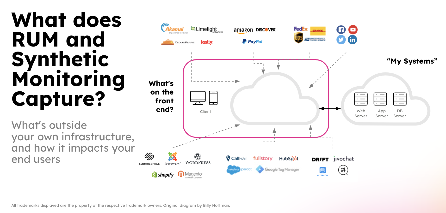
Use Splunk Real User Monitoring (RUM) and Synthetics to get insight into end user experience, and proactively test scenarios to improve that experience.
Deploy ThousandEyes Enterprise Agent in Kubernetes, stream synthetic data into Splunk Observability Cloud, and enable bi-directional drilldowns between ThousandEyes and Splunk APM.
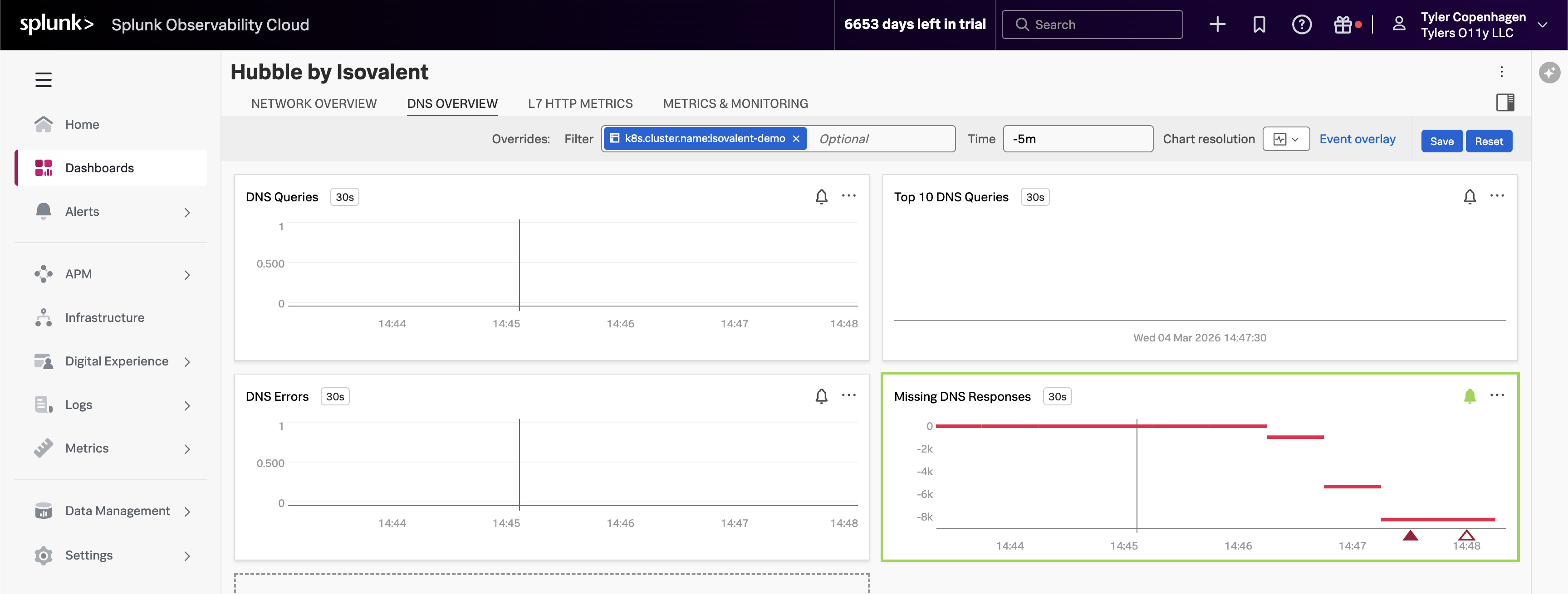
Deploy Isovalent Enterprise Platform (Cilium, Hubble, and Tetragon) on Amazon EKS and integrate with Splunk Observability Cloud for comprehensive eBPF-based monitoring and observability. Includes an end-to-end demo investigating a DNS issue using Hubble dashboards.
Integrate Cisco Catalyst Center, Solarwinds, and Splunk ITSI to correlate network events across vendors, reduce alert noise, and understand the business impact of network incidents.
Subsections of Scenarios
Optimize Cloud Monitoring
3 minutesAuthor
Tim Hard
The elasticity of cloud architectures means that monitoring artifacts must scale elastically as well, breaking the paradigm of purpose-built monitoring assets. As a result, administrative overhead, visibility gaps, and tech debt skyrocket while MTTR slows. This typically happens for three reasons:
Complex and Inefficient Data Management: Infrastructure data is scattered across multiple tools with inconsistent naming conventions, leading to fragmented views and poor metadata and labelling. Managing multiple agents and data flows adds to the complexity.
Inadequate Monitoring and Troubleshooting Experience: Slow data visualization and troubleshooting, cluttered with bespoke dashboards and manual correlations, are hindered further by the lack of monitoring tools for ephemeral technologies like Kubernetes and serverless functions.
Operational and Scaling Challenges: Manual onboarding, user management, and chargeback processes, along with the need for extensive data summarization, slow down operations and inflate administrative tasks, complicating data collection and scalability.
To address these challenges you need a way to:
Standardize Data Collection and Tags: Centralized monitoring with a single, open-source agent to apply uniform naming standards and ensure metadata for visibility. Optimize data collection and use a monitoring-as-code approach for consistent collection and tagging.
Reuse Content Across Teams: Streamline new IT infrastructure onboarding and user management with templates and automation. Utilize out-of-the-box dashboards, alerts, and self-service tools to enable content reuse, ensuring uniform monitoring and reducing manual effort.
Improve Timeliness of Alerts: Utilize highly performant open source data collection, combined with real-time streaming-based data analytics and alerting, to enhance the timeliness of notifications. Automatically configured alerts for common problem patterns (AutoDetect) and minimal yet effective monitoring dashboards and alerts will ensure rapid response to emerging issues, minimizing potential disruptions.
Correlate Infrastructure Metrics and Logs: Achieve full monitoring coverage of all IT infrastructure by enabling seamless correlation between infrastructure metrics and logs. High-performing data visualization and a single source of truth for data, dashboards, and alerts will simplify the correlation process, allowing for more effective troubleshooting and analysis of the IT environment.
In this workshop, we’ll explore:
How to standardize data collection and tags using OpenTelemetry.
How to reuse content across teams.
How to improve timelines of alerts.
How to correlate infrastructure metrics and logs.
Tip
The easiest way to navigate through this workshop is by using:
the left/right arrows (< | >) on the top right of this page
the left (◀️) and right (▶️) cursor keys on your keyboard
Subsections of Optimize Cloud Monitoring
Getting Started
3 minutesAuthor
Tim Hard
During this technical Optimize Cloud Monitoring Workshop, you will build out an environment based on a lightweight Kubernetes1 cluster.
To simplify the workshop modules, a pre-configured AWS/EC2 instance is provided.
The instance is pre-configured with all the software required to deploy the Splunk OpenTelemetry Connector2 and the microservices-based OpenTelemetry Demo Application3 in Kubernetes which has been instrumented using OpenTelemetry to send metrics, traces, spans and logs.
This workshop will introduce you to the benefits of standardized data collection, how content can be re-used across teams, correlating metrics and logs, and creating detectors to fire alerts. By the end of these technical workshops, you will have a good understanding of some of the key features and capabilities of the Splunk Observability Cloud.
Here are the instructions on how to access your pre-configured AWS/EC2 instance
Kubernetes is a portable, extensible, open-source platform for managing containerized workloads and services, that facilitates both declarative configuration and automation. ↩︎
OpenTelemetry Collector offers a vendor-agnostic implementation on how to receive, process and export telemetry data. In addition, it removes the need to run, operate and maintain multiple agents/collectors to support open-source telemetry data formats (e.g. Jaeger, Prometheus, etc.) sending to multiple open-source or commercial back-ends. ↩︎
The OpenTelemetry Demo Application is a microservice-based distributed system intended to illustrate the implementation of OpenTelemetry in a near real-world environment. ↩︎
Subsections of 1. Getting Started
How to connect to your workshop environment
5 minutesAuthor
Tim Hard
How to retrieve the IP address of the AWS/EC2 instance assigned to you.
Connect to your instance using SSH, Putty1 or your web browser.
Verify your connection to your AWS/EC2 cloud instance.
Using Putty (Optional)
Using Multipass (Optional)
1. AWS/EC2 IP Address
In preparation for the workshop, Splunk has prepared an Ubuntu Linux instance in AWS/EC2.
To get access to the instance that you will be using in the workshop please visit the URL to access the Google Sheet provided by the workshop leader.
Search for your AWS/EC2 instance by looking for your first and last name, as provided during registration for this workshop.
Find your allocated IP address, SSH command (for Mac OS, Linux and the latest Windows versions) and password to enable you to connect to your workshop instance.
It also has the Browser Access URL that you can use in case you cannot connect via SSH or Putty - see EC2 access via Web browser
Important
Please use SSH or Putty to gain access to your EC2 instance if possible and
make a note of the IP address as you will need this during the workshop.
2. SSH (Mac OS/Linux)
Most attendees will be able to connect to the workshop by using SSH from their Mac or Linux device, or on Windows 10 and above.
To use SSH, open a terminal on your system and type ssh splunk@x.x.x.x (replacing x.x.x.x with the IP address found in Step #1).
When prompted Are you sure you want to continue connecting (yes/no/[fingerprint])? please type yes.
Enter the password provided in the Google Sheet from Step #1.
Upon successful login, you will be presented with the Splunk logo and the Linux prompt.
3. SSH (Windows 10 and above)
The procedure described above is the same on Windows 10, and the commands can be executed either in the Windows Command Prompt or PowerShell.
However, Windows regards its SSH Client as an “optional feature”, which might need to be enabled.
You can verify if SSH is enabled by simply executing ssh
If you are shown a help text on how to use the SSH command (like shown in the screenshot below), you are all set.
If the result of executing the command looks something like the screenshot below, you want to enable the “OpenSSH Client” feature manually.
To do that, open the “Settings” menu, and click on “Apps”. While in the “Apps & features” section, click on “Optional features”.
Here, you are presented with a list of installed features. On the top, you see a button with a plus icon to “Add a feature”. Click it.
In the search input field, type “OpenSSH”, and find a feature called “OpenSSH Client”, or respectively, “OpenSSH Client (Beta)”, click on it, and click the “Install”-button.
Now you are set! In case you are not able to access the provided instance despite enabling the OpenSSH feature, please do not shy away from reaching
out to the course instructor, either via chat or directly.
If you are blocked from using SSH (Port 22) or unable to install Putty you may be able to connect to the workshop instance by using a web browser.
Note
This assumes that access to port 6501 is not restricted by your company’s firewall.
Open your web browser and type http://x.x.x.x:6501 (where X.X.X.X is the IP address from the Google Sheet).
Once connected, login in as splunk and the password is the one provided in the Google Sheet.
Once you are connected successfully you should see a screen similar to the one below:
Unlike when you are using regular SSH, copy and paste does require a few extra steps to complete when using a browser session. This is due to cross browser restrictions.
When the workshop asks you to copy instructions into your terminal, please do the following:
Copy the instruction as normal, but when ready to paste it in the web terminal, choose Paste from the browser as show below:
This will open a dialogue box asking for the text to be pasted into the web terminal:
Paste the text in the text box as shown, then press OK to complete the copy and paste process.
Note
Unlike regular SSH connection, the web browser has a 60-second time out, and you will be disconnected, and a Connect button will be shown in the center of the web terminal.
Simply click the Connect button and you will be reconnected and will be able to continue.
For this workshop, we’ll be using the OpenTelemetry Demo Application running in Kubernetes. This application is for an online retailer and includes more than a dozen services written in many different languages. While metrics, traces, and logs are being collected from this application, this workshop is primarily focused on how Splunk Observability Cloud can be used to more efficiently monitor infrastructure.
The initial setup can be completed by executing the following steps on the command line of your EC2 instance.
cd ~/workshop/optimize-cloud-monitoring &&\
./deploy-application.sh
You’ll be asked to enter your favorite city. This will be used in the OpenTelemetry Collector configuration as a custom tag to show how easy it is to add additional context to your observability data.
Your application should now be running and sending data to Splunk Observability Cloud. You’ll dig into the data in the next section.
Standardize Data Collection
2 minutesAuthor
Tim Hard
Why Standards Matter
As cloud adoption grows, we often face requests to support new technologies within a diverse landscape, posing challenges in delivering timely content. Take, for instance, a team containerizing five workloads on AWS requiring EKS visibility. Usually, this involves assisting with integration setup, configuring metadata, and creating dashboards and alerts—a process that’s both time-consuming and increases administrative overhead and technical debt.
Splunk Observability Cloud was designed to handle customers with a diverse set of technical requirements and stacks – from monolithic to microservices architectures, from homegrown applications to Software-as-a-Service.
Splunk offers a native experience for OpenTelemetry, which means OTel is the preferred way to get data into Splunk.
Between Splunk’s integrations and the OpenTelemetry community, there are a number of integrations available to easily collect from diverse infrastructure and applications. This includes both on-prem systems like VMWare and as well as guided integrations with cloud vendors, centralizing these hybrid environments.
For someone like a Splunk admin, the OpenTelemetry Collector can additionally be deployed to a Splunk Universal Forwarder as a Technical Add-on. This enables fast roll-out and centralized configuration management using the Splunk Deployment Server.
Let’s assume that the same team adopting Kubernetes is going to deploy a cluster for each one of our B2B customers. I’ll show you how to make a simple modification to the OpenTelemetry collector to add the customerID, and then use mirrored dashboards to allow any of our SRE teams to easily see the customer they care about.
Subsections of 2. Standardize Data Collection
What Are Tags?
3 minutesAuthor
Tim Hard
Tags are key-value pairs that provide additional metadata about metrics, spans in a trace, or logs allowing you to enrich the context of the data you send to Splunk Observability Cloud. Many tags are collected by default such as hostname or OS type. Custom tags can be used to provide environment or application-specific context. Examples of custom tags include:
Infrastructure specific attributes
What data center a host is in
What services are hosted on an instance
What team is responsible for a set of hosts
Application specific attributes
What Application Version is running
Feature flags or experimental identifiers
Tenant ID in multi-tenant applications
User related attributes
User ID
User role (e.g. admin, guest, subscriber)
User geographical location (e.g. country, city, region)
There are two ways to add tags to your data
Add tags as OpenTelemetry attributes to metrics, traces, and logs when you send data to the Splunk Distribution of OpenTelemetry Collector. This option lets you add spans in bulk.
Instrument your application to create span tags. This option gives you the most flexibility at the per-application level.
Why are tags so important?
Tags are essential for an application to be truly observable. Tags add context to the traces to help us understand why some users get a great experience and others don’t. Powerful features in Splunk Observability Cloud utilize tags to help you jump quickly to the root cause.
Contextual Information: Tags provide additional context to the metrics, traces, and logs allowing developers and operators to understand the behavior and characteristics of infrastructure and traced operations.
Filtering and Aggregation: Tags enable filtering and aggregation of collected data. By attaching tags, users can filter and aggregate data based on specific criteria. This filtering and aggregation help in identifying patterns, diagnosing issues, and gaining insights into system behavior.
Correlation and Analysis: Tags facilitate correlation between metrics and other telemetry data, such as traces and logs. By including common identifiers or contextual information as tags, users can correlate metrics, traces, and logs enabling comprehensive analysis and troubleshooting of distributed systems.
Customization and Flexibility: OpenTelemetry allows developers to define custom tags based on their application requirements. This flexibility enables developers to capture domain-specific metadata or contextual information that is crucial for understanding the behavior of their applications.
Attributes vs. Tags
A note about terminology before we proceed. While this workshop is about tags, and this is the terminology we use in Splunk Observability Cloud, OpenTelemetry uses the term attributes instead. So when you see tags mentioned throughout this workshop, you can treat them as synonymous with attributes.
For this workshop, the OpenTelemetry collector is pre-configured to use the city you provided as a custom tag called store.location which will be used to emulate Kubernetes Clusters running in different geographic locations. We’ll use this tag as a filter to show how you can use Out-of-the-Box integration dashboards to quickly create views for specific teams, applications, or other attributes about your environment. Efficiently enabling content to be reused across teams without increasing technical debt.
Here is the OpenTelemetry Collector configuration used to add the store.location tag to all of the data sent to this collector. This means any metrics, traces, or logs will contain the store.location tag which can then be used to search, filter, or correlate this value.
Tip
If you’re interested in a deeper dive on the OpenTelemetry Collector, head over to the Self Service Observability workshop where you can get hands-on with configuring the collector or the OpenTelemetry Collector Ninja Workshop where you’ll dissect the inner workings of each collector component.
While this example uses a hard-coded value for the tag, parameterized values can also be used, allowing you to customize the tags dynamically based on the context of each host, application, or operation. This flexibility enables you to capture relevant metadata, user-specific details, or system parameters, providing a rich context for metrics, tracing, and log data while enhancing the observability of your distributed systems.
Now that you have the appropriate context, which as we’ve established is critical to Observability, let’s head over to Splunk Observability Cloud and see how we can use the data we’ve just configured.
Reuse Content Across Teams
3 minutesAuthor
Tim Hard
In today’s rapidly evolving technological landscape, where hybrid and cloud environments are becoming the norm, the need for effective monitoring and troubleshooting solutions has never been more critical. However, managing the elasticity and complexity of these modern infrastructures poses a significant challenge for teams across various industries. One of the primary pain points encountered in this endeavor is the inadequacy of existing monitoring and troubleshooting experiences.
Traditional monitoring approaches often fall short in addressing the intricacies of hybrid and cloud environments. Teams frequently encounter slow data visualization and troubleshooting processes, compounded by the clutter of bespoke yet similar dashboards and the manual correlation of data from disparate sources. This cumbersome workflow is made worse by the absence of monitoring tools tailored to ephemeral technologies such as containers, orchestrators like Kubernetes, and serverless functions.
In this section, we’ll cover how Splunk Observability Cloud provides out-of-the-box content for every integration. Not only do the out-of-the-box dashboards provide rich visibility into the infrastructure that is being monitored they can also be mirrored. This is important because it enables you to create standard dashboards for use by teams throughout your organization. This allows all teams to see any changes to the charts in the dashboard, and members of each team can set dashboard variables and filter customizations relevant to their requirements.
Subsections of 3. Reuse Content Across Teams
Infrastrcuture Navigators
5 minutesAuthor
Tim Hard
Splunk Infrastructure Monitoring (IM) is a market-leading monitoring and observability service for hybrid cloud environments. Built on a patented streaming architecture, it provides a real-time solution for engineering teams to visualize and analyze performance across infrastructure, services, and applications in a fraction of the time and with greater accuracy than traditional solutions.
300+ Easy-to-use OOTB content: Pre-built navigators and dashboards, deliver immediate visualizations of your entire environment so that you can interact with all your data in real time. Kubernetes navigator: Provides an instant, comprehensive out-of-the-box hierarchical view of nodes, pods, and containers. Ramp up even the most novice Kubernetes user with easy-to-understand interactive cluster maps. AutoDetect alerts and detectors: Automatically identify the most important metrics, out-of-the-box, to create alert conditions for detectors that accurately alert from the moment telemetry data is ingested and use real-time alerting capabilities for important notifications in seconds. Log views in dashboards: Combine log messages and real-time metrics on one page with common filters and time controls for faster in-context troubleshooting. Metrics pipeline management: Control metrics volume at the point of ingest without re-instrumentation with a set of aggregation and data-dropping rules to store and analyze only the needed data. Reduce metrics volume and optimize observability spend.
Exercise: Find your Kubernetes Cluster
From the Splunk Observability Cloud homepage, click the button -> Kubernetes -> K8s nodes
First, use the option to pick your cluster.
From the filter drop-down box, use the store.location value you entered when deploying the application.
You then can start typing the city you used which should also appear in the drop-down values. Select yours and make sure just the one for your workshop is highlighted with a .
Click the Apply Filter button to focus on our Cluster.
You should now have your Kubernetes Cluster visible
Here we can see all of the different components of the cluster (Nodes, Pods, etc), each of which has relevant metrics associated with it. On the right side, you can also see what services are running in the cluster.
Before moving to the next section, take some time to explore the Kubernetes Navigator to see the data that is available Out of the Box.
Dashboard Cloning
5 minutesAuthor
Tim Hard
ITOps teams responsible for monitoring fleets of infrastructure frequently find themselves manually creating dashboards to visualize and analyze metrics, traces, and log data emanating from rapidly changing cloud-native workloads hosted in Kubernetes and serverless architectures, alongside existing on-premises systems. Moreover, due to the absence of a standardized troubleshooting workflow, teams often resort to creating numerous custom dashboards, each resembling the other in structure and content. As a result, administrative overhead skyrockets and MTTR slows.
To address this, you can use the out-of-the-box dashboards available in Splunk Observability Cloud for each and every integration. These dashboards are filterable and can be used for ad hoc troubleshooting or as a templated approach to getting users the information they need without having to start from scratch. Not only do the out-of-the-box dashboards provide rich visibility into the infrastructure that is being monitored they can also be cloned.
Exercise: Create a Mirrored Dashboard
In Splunk Observability Cloud, click the Global Search button. (Global Search can be used to quickly find content)
Search for Pods and select K8s pods (Kubernetes)
This will take you to the out-of-the-box Kubernetes Pods dashboard which we will use as a template for mirroring dashboards.
In the upper right corner of the dashboard click the Dashboard actions button (3 horizontal dots) -> Click Save As…
Enter a dashboard name (i.e. Kubernetes Pods Dashboard)
Under Dashboard group search for your e-mail address and select it.
Click Save
Note: Every Observability Cloud user who has set a password and logged in at least once, gets a user dashboard group and user dashboard. Your user dashboard group is your individual workspace within Observability Cloud.
After saving, you will be taken to the newly created dashboard in the Dashboard Group for your user. This is an example of cloning an out-of-the-box dashboard which can be further customized and enables users to quickly build role, application, or environment relevant views.
Custom dashboards are meant to be used by multiple people and usually represent a curated set of charts that you want to make accessible to a broad cross-section of your organization. They are typically organized by service, team, or environment.
Dashboard Mirroring
5 minutesAuthor
Tim Hard
Not only do the out-of-the-box dashboards provide rich visibility into the infrastructure that is being monitored they can also be mirrored. This is important because it enables you to create standard dashboards for use by teams throughout your organization. This allows all teams to see any changes to the charts in the dashboard, and members of each team can set dashboard variables and filter customizations relevant to their requirements.
Exercise: Create a Mirrored Dashboard
While on the Kubernetes Pods dashboard, you created in the previous step, In the upper right corner of the dashboard click the Dashboard actions button (3 horizontal dots) -> Click Add a mirror…. A configuration modal for the Dashboard Mirror will open.
Under My dashboard group search for your e-mail address and select it.
(Optional) Modify the dashboard in Dashboard name override name.
(Optional) Add a dashboard description in Dashboard description override.
Under Default filter overrides search for k8s.cluster.name and select the name of your Kubernetes cluster.
Under Default filter overrides search for store.location and select the city you entered during the workshop setup.
Click Save
You will now be taken to the newly created dashboard which is a mirror of the Kubernetes Pods dashboard you created in the previous section. Any changes to the original dashboard will be reflected in this dashboard as well. This allows teams to have a consistent yet specific view of the systems they care about and any modifications or updates can be applied in a single location, significantly minimizing the effort needed when compared to updating each individual dashboard.
In the next section, you’ll add a new logs-based chart to the original dashboard and see how the dashboard mirror is automatically updated as well.
Correlate Metrics and Logs
1 minuteAuthor
Tim Hard
Correlating infrastructure metrics and logs is often a challenging task, primarily due to inconsistencies in naming conventions across various data sources, including hosts operating on different systems. However, leveraging the capabilities of OpenTelemetry can significantly simplify this process. With OpenTelemetry’s robust framework, which offers rich metadata and attribution, metrics, traces, and logs can seamlessly correlate using standardized field names. This automated correlation not only alleviates the burden of manual effort but also enhances the overall observability of the system.
By aligning metrics and logs based on common field names, teams gain deeper insights into system performance, enabling more efficient troubleshooting, proactive monitoring, and optimization of resources. In this workshop section, we’ll explore the importance of correlating metrics with logs and demonstrate how Splunk Observability Cloud empowers teams to unlock additional value from their observability data.
Subsections of 4. Correlate Metrics and Logs
Correlate Metrics and Logs
5 minutesAuthor
Tim Hard
In this section, we’ll dive into the seamless correlation of metrics and logs facilitated by the robust naming standards offered by OpenTelemetry. By harnessing the power of OpenTelemetry within Splunk Observability Cloud, we’ll demonstrate how troubleshooting issues becomes significantly more efficient for Site Reliability Engineers (SREs) and operators. With this integration, contextualizing data across various telemetry sources no longer demands manual effort to correlate information. Instead, SREs and operators gain immediate access to the pertinent context they need, allowing them to swiftly pinpoint and resolve issues, improving system reliability and performance.
Exercise: View pod logs
The Kubernetes Pods Dashboard you created in the previous section already includes a chart that contains all of the pod logs for your Kubernetes Cluster. The log entries are split by container in this stacked bar chart. To view specific log entries perform the following steps:
On the Kubernetes Pods Dashboard click on one of the bar charts. A modal will open with the most recent log entries for the container you’ve selected.
Click one of the log entries.
Here we can see the entire log event with all of the fields and values. You can search for specific field names or values within the event itself using the Search for fields bar in the event.
Enter the city you configured during the application deployment
The event will now be filtered to the store.location field. This feature is great for exploring large log entries for specific fields and values unique to your environment or to search for keywords like Error or Failure.
Close the event using the X in the upper right corner.
Click the Chart actions (three horizontal dots) on the Pod log event rate chart
Click View in Log Observer
This will take us to Log Observer. In the next section, you’ll create a chart based on log events and add it to the K8s Pod Dashboard you cloned in section 3.2 Dashboard Cloning. You’ll also see how this new chart is automatically added to the mirrored dashboard you created in section 3.3 Dashboard Mirroring.
Create Log-based Chart
5 minutesAuthor
Tim Hard
In Log Observer, you can perform codeless queries on logs to detect the source of problems in your systems. You can also extract fields from logs to set up log processing rules and transform your data as it arrives or send data to Infinite Logging S3 buckets for future use. See What can I do with Log Observer? to learn more about Log Observer capabilities.
In this section, you’ll create a chart filtered to logs that include errors which will be added to the K8s Pod Dashboard you cloned in section 3.2 Dashboard Cloning.
Exercise: Create Log-based Chart
Because you drilled into Log Observer from the K8s Pod Dashboard in the previous section, the dashboard will already be filtered to your cluster and store location using the k8s.cluster.name and store.location fields and the bar chart is split by k8s.pod.name. To filter the dashboard to only logs that contain errors complete the following steps:
Log Observer can be filtered using Keywords or specific key-value pairs.
In Log Observer click Add Filter along the top.
Make sure you’ve selected Fields as the filter type and enter severity in the Find a field… search bar.
Select severity from the fields list.
You should now see a list of severities and the number of log entries for each.
Under Top values, hover over Error and click the = button to apply the filter.
The dashboard will now be filtered to only log entries with a severity of Error and the bar chart will be split by the Kubernetes Pod that contains the errors. Next, you’ll save the chart on your Kubernetes Pods Dashboard.
In the upper right corner of the Log Observer dashboard click Save.
Select Save to Dashboard.
In the Chart name field enter a name for your chart.
(Optional) In the Chart description field enter a description for your chart.
Click Select Dashboard and search for the name of the Dashboard you cloned in section 3.2 Dashboard Cloning.
Select the dashboard in the Dashboard Group for your email address.
Click OK
For the Chart type select Log timeline
Click Save and go to the dashboard
You will now be taken to your Kubernetes Pods Dashboard where you should see the chart you just created for pod errors.
Because you updated the original Kubernetes Pods Dashboard, your mirrored dashboard will also include this chart as well! You can see this by clicking the mirrored version of your dashboard along the top of the Dashboard Group for your user.
Now that you’ve seen how data can be reused across teams by cloning the dashboard, creating dashboard mirrors and how metrics can easily be correlated with logs, let’s take a look at how to create alerts so your teams can be notified when there is an issue with their infrastructure, services, or applications.
Improve Timeliness of Alerts
1 minutesAuthor
Tim Hard
When monitoring hybrid and cloud environments, ensuring timely alerts for critical infrastructure and applications poses a significant challenge. Typically, this involves crafting intricate queries, meticulously scheduling searches, and managing alerts across various monitoring solutions. Moreover, the proliferation of disparate alerts generated from identical data sources often results in unnecessary duplication, contributing to alert fatigue and noise within the monitoring ecosystem.
In this section, we’ll explore how Splunk Observability Cloud addresses these challenges by enabling the effortless creation of alert criteria. Leveraging its 10-second default data collection capability, alerts can be triggered swiftly, surpassing the timeliness achieved by traditional monitoring tools. This enhanced responsiveness not only reduces Mean Time to Detect (MTTD) but also accelerates Mean Time to Resolve (MTTR), ensuring that critical issues are promptly identified and remediated.
Subsections of 5. Improve Timeliness of Alerts
Create Custom Detector
10 minutesAuthor
Tim Hard
Splunk Observability Cloud provides detectors, events, alerts, and notifications to keep you informed when certain criteria are met. There are a number of pre-built AutoDetect Detectors that automatically surface when common problem patterns occur, such as when an EC2 instance’s CPU utilization is expected to reach its limit. Additionally, you can also create custom detectors if you want something more optimized or specific. For example, you want a message sent to a Slack channel or to an email address for the Ops team that manages this Kubernetes cluster when Memory Utilization on their pods has reached 85%.
Exercise: Create Custom Detector
In this section you’ll create a detector on Pod Memory Utilization which will trigger if utilization surpasses 85%
On the Kubernetes Pods Dashboard you cloned in section 3.2 Dashboard Cloning, click the Get Alerts button (bell icon) for the Memory usage (%) chart -> Click New detector from chart.
In the Create detector add your initials to the detector name.
Click Create alert rule.
These conditions are expressed as one or more rules that trigger an alert when the conditions in the rules are met. Importantly, multiple rules can be included in the same detector configuration which minimizes the total number of alerts that need to be created and maintained. You can see which signal this detector will alert on by the bell icon in the Alert On column. In this case, this detector will alert on the Memory Utilization for the pods running in this Kubernetes cluster.
Click Proceed To Alert Conditions.
Many pre-built alert conditions can be applied to the metric you want to alert on. This could be as simple as a static threshold or something more complex, for example, is memory usage deviating from the historical baseline across any of your 50,000 containers?
Select Static Threshold.
Click Proceed To Alert Settings.
In this case, you want the alert to trigger if any pods exceed 85% memory utilization. Once you’ve set the alert condition, the configuration is back-tested against the historical data so you can confirm that the alert configuration is accurate, meaning will the alert trigger on the criteria you’ve defined? This is also a great way to confirm if the alert generates too much noise.
Enter 85 in the Threshold field.
Click Proceed To Alert Message.
Next, you can set the severity for this alert, you can include links to runbooks and short tips on how to respond, and you can customize the message that is included in the alert details. The message can include parameterized fields from the actual data, for example, in this case, you may want to include which Kubernetes node the pod is running on, or the store.location configured when you deployed the application, to provide additional context.
Click Proceed To Alert Recipients.
You can choose where you want this alert to be sent when it triggers. This could be to a team, specific email addresses, or to other systems such as ServiceNow, Slack, Splunk On-Call or Splunk ITSI. You can also have the alert execute a webhook which enables me to leverage automation or to integrate with many other systems such as homegrown ticketing tools. For the purpose of this workshop do not include a recipient
Click Proceed To Alert Activation.
Click Activate Alert.
You will receive a warning because no recipients were included in the Notification Policy for this detector. This can be warning can be dismissed.
Click Save.
You will be taken to your newly created detector where you can see any triggered alerts.
In the upper right corner, Click Close to close the Detector.
The detector status and any triggered alerts will automatically be included in the chart because this detector was configured for this chart.
Congratulations! You’ve successfully created a detector that will trigger if pod memory utilization exceeds 85%. After a few minutes, the detector should trigger some alerts. You can click the detector name in the chart to view the triggered alerts.
Conclusion
1 minute
Today you’ve seen how Splunk Observability Cloud can help you overcome many of the challenges you face monitoring hybrid and cloud environments. You’ve demonstrated how Splunk Observability Cloud streamlines operations with standardized data collection and tags, ensuring consistency across all IT infrastructure. The Unified Service Telemetry has been a game-changer, providing in-context metrics, logs, and trace data that make troubleshooting swift and efficient. By enabling the reuse of content across teams, you’re minimizing technical debt and bolstering the performance of our monitoring systems.
This workshop shows how tags can be used to reduce the time required for SREs to isolate issues across services, so they know which team to engage to troubleshoot the issue further, and can provide context to help engineering get a head start on debugging.
This workshop shows how Database Query Performance and AlwaysOn Profiling can be used to reduce the time required for engineers to debug problems in microservices.
Subsections of Debug Problems in Microservices
Tagging Workshop
2 minutesAuthor
Derek Mitchell
Splunk Observability Cloud includes powerful features that dramatically reduce the time required for SREs to isolate issues across services, so they know which team to engage to troubleshoot the issue further, and can provide context to help engineering get a head start on debugging.
Unlocking these features requires tags to be included with your application traces. But how do you know which tags are the most valuable and how do you capture them?
In this workshop, we’ll explore:
What are tags and why are they such a critical part of making an application observable.
How to use OpenTelemetry to capture tags of interest from your application.
How to index tags in Splunk Observability Cloud and the differences between Troubleshooting MetricSets and Monitoring MetricSets.
How to utilize tags in Splunk Observability Cloud to find “unknown unknowns” using the Tag Spotlight and Dynamic Service Map features.
How to utilize tags for alerting and dashboards.
The workshop uses a simple microservices-based application to illustrate these concepts. Let’s get started!
Tip
The easiest way to navigate through this workshop is by using:
the left/right arrows (< | >) on the top right of this page
the left (◀️) and right (▶️) cursor keys on your keyboard
Subsections of Tagging Workshop
Build the Sample Application
10 minutes
Introduction
For this workshop, we’ll be using a microservices-based application. This application is for an online retailer and normally includes more than a dozen services. However, to keep the workshop simple, we’ll be focusing on two services used by the retailer as part of their payment processing workflow: the credit check service and the credit processor service.
Pre-requisites
You will start with an EC2 instance and perform some initial steps in order to get to the following state:
Deploy the Splunk distribution of the OpenTelemetry Collector
Build and deploy creditcheckservice and creditprocessorservice
Deploy a load generator to send traffic to the services
Initial Steps
The initial setup can be completed by executing the following steps on the command line of your EC2 instance:
cd workshop/tagging
./0-deploy-collector-with-services.sh
Java
There are implementations in multiple languages available for creditcheckservice.
Run
./0-deploy-collector-with-services.sh java
to pick Java over Python.
View your application in Splunk Observability Cloud
Now that the setup is complete, let’s confirm that it’s sending data to Splunk Observability Cloud. Note that when the application is deployed for the first time, it may take a few minutes for the data to appear.
Navigate to APM, then use the Environment dropdown to select your environment (i.e. tagging-workshop-instancename).
If everything was deployed correctly, you should see creditprocessorservice and creditcheckservice displayed in the list of services:
Click on Service Map on the right-hand side to view the service map. We can see that the creditcheckservice makes calls to the creditprocessorservice, with an average response time of at least 3 seconds:
Next, click on Traces on the right-hand side to see the traces captured for this application. You’ll see that some traces run relatively fast (i.e. just a few milliseconds), whereas others take a few seconds.
If you toggle Errors only to on, you’ll also notice that some traces have errors:
Toggle Errors only back to off and sort the traces by duration, then click on one of the longer running traces. In this example, the trace took five seconds, and we can see that most of the time was spent calling the /runCreditCheck operation, which is part of the creditprocessorservice.
Currently, we don’t have enough details in our traces to understand why some requests finish in a few milliseconds, and others take several seconds. To provide the best possible customer experience, this will be critical for us to understand.
We also don’t have enough information to understand why some requests result in errors, and others don’t. For example, if we look at one of the error traces, we can see that the error occurs when the creditprocessorservice attempts to call another service named otherservice. But why do some requests results in a call to otherservice, and others don’t?
We’ll explore these questions and more in the workshop.
What are Tags?
3 minutes
To understand why some requests have errors or slow performance, we’ll need to add context to our traces. We’ll do this by adding tags. But first, let’s take a moment to discuss what tags are, and why they’re so important for observability.
What are tags?
Tags are key-value pairs that provide additional metadata about spans in a trace, allowing you to enrich the context of the spans you send to Splunk APM.
For example, a payment processing application would find it helpful to track:
The payment type used (i.e. credit card, gift card, etc.)
The ID of the customer that requested the payment
This way, if errors or performance issues occur while processing the payment, we have the context we need for troubleshooting.
While some tags can be added with the OpenTelemetry collector, the ones we’ll be working with in this workshop are more granular, and are added by application developers using the OpenTelemetry API.
Attributes vs. Tags
A note about terminology before we proceed. While this workshop is about tags, and this is the terminology we use in Splunk Observability Cloud, OpenTelemetry uses the term attributes instead. So when you see tags mentioned throughout this workshop, you can treat them as synonymous with attributes.
Why are tags so important?
Tags are essential for an application to be truly observable. As we saw with our credit check service, some users are having a great experience: fast with no errors. But other users get a slow experience or encounter errors.
Tags add the context to the traces to help us understand why some users get a great experience and others don’t. And powerful features in Splunk Observability Cloud utilize tags to help you jump quickly to root cause.
Sneak Peak: Tag Spotlight
Tag Spotlight uses tags to discover trends that contribute to high latency or error rates:
The screenshot above provides an example of Tag Spotlight from another application.
Splunk has analyzed all of the tags included as part of traces that involve the payment service.
It tells us very quickly whether some tag values have more errors than others.
If we look at the version tag, we can see that version 350.10 of the service has a 100% error rate, whereas version 350.9 of the service has no errors at all:
We’ll be using Tag Spotlight with the credit check service later on in the workshop, once we’ve captured some tags of our own.
Capture Tags with OpenTelemetry
15 minutes
Please proceed to one of the subsections for Java or Python. Ask your instructor for the one used during the workshop!
Subsections of 3. Capture Tags with OpenTelemetry
1. Capture Tags - Java
15 minutes
Let’s add some tags to our traces, so we can find out why some customers receive a poor experience from our application.
Identify Useful Tags
We’ll start by reviewing the code for the creditCheck function of creditcheckservice (which can be found in the file /home/splunk/workshop/tagging/creditcheckservice-java/src/main/java/com/example/creditcheckservice/CreditCheckController.java):
@GetMapping("/check")publicResponseEntity<String>creditCheck(@RequestParam("customernum")StringcustomerNum){// Get Credit ScoreintcreditScore;try{StringcreditScoreUrl="http://creditprocessorservice:8899/getScore?customernum="+customerNum;creditScore=Integer.parseInt(restTemplate.getForObject(creditScoreUrl,String.class));}catch(HttpClientErrorExceptione){returnResponseEntity.status(HttpStatus.INTERNAL_SERVER_ERROR).body("Error getting credit score");}StringcreditScoreCategory=getCreditCategoryFromScore(creditScore);// Run Credit CheckStringcreditCheckUrl="http://creditprocessorservice:8899/runCreditCheck?customernum="+customerNum+"&score="+creditScore;StringcheckResult;try{checkResult=restTemplate.getForObject(creditCheckUrl,String.class);}catch(HttpClientErrorExceptione){returnResponseEntity.status(HttpStatus.INTERNAL_SERVER_ERROR).body("Error running credit check");}returnResponseEntity.ok(checkResult);}
We can see that this function accepts a customer number as an input. This would be helpful to capture as part of a trace. What else would be helpful?
Well, the credit score returned for this customer by the creditprocessorservice may be interesting (we want to ensure we don’t capture any PII data though). It would also be helpful to capture the credit score category, and the credit check result.
Great, we’ve identified four tags to capture from this service that could help with our investigation. But how do we capture these?
Capture Tags
We start by adding OpenTelemetry imports to the top of the CreditCheckController.java file:
That was pretty easy, right? Let’s capture some more, with the final result looking like this:
@GetMapping("/check")@WithSpan(kind=SpanKind.SERVER)publicResponseEntity<String>creditCheck(@RequestParam("customernum")@SpanAttribute("customer.num")StringcustomerNum){// Get Credit ScoreintcreditScore;try{StringcreditScoreUrl="http://creditprocessorservice:8899/getScore?customernum="+customerNum;creditScore=Integer.parseInt(restTemplate.getForObject(creditScoreUrl,String.class));}catch(HttpClientErrorExceptione){returnResponseEntity.status(HttpStatus.INTERNAL_SERVER_ERROR).body("Error getting credit score");}SpancurrentSpan=Span.current();currentSpan.setAttribute("credit.score",creditScore);StringcreditScoreCategory=getCreditCategoryFromScore(creditScore);currentSpan.setAttribute("credit.score.category",creditScoreCategory);// Run Credit CheckStringcreditCheckUrl="http://creditprocessorservice:8899/runCreditCheck?customernum="+customerNum+"&score="+creditScore;StringcheckResult;try{checkResult=restTemplate.getForObject(creditCheckUrl,String.class);}catch(HttpClientErrorExceptione){returnResponseEntity.status(HttpStatus.INTERNAL_SERVER_ERROR).body("Error running credit check");}currentSpan.setAttribute("credit.check.result",checkResult);returnResponseEntity.ok(checkResult);}
Redeploy Service
Once these changes are made, let’s run the following script to rebuild the Docker image used for creditcheckservice and redeploy it to our Kubernetes cluster:
./5-redeploy-creditcheckservice.sh java
Confirm Tag is Captured Successfully
After a few minutes, return to Splunk Observability Cloud and load one of the latest traces to confirm that the tags were captured successfully (hint: sort by the timestamp to find the latest traces):
Well done, you’ve leveled up your OpenTelemetry game and have added context to traces using tags.
Next, we’re ready to see how you can use these tags with Splunk Observability Cloud!
2. Capture Tags - Python
15 minutes
Let’s add some tags to our traces, so we can find out why some customers receive a poor experience from our application.
Identify Useful Tags
We’ll start by reviewing the code for the credit_check function of creditcheckservice (which can be found in the /home/splunk/workshop/tagging/creditcheckservice-py/main.py file):
@app.route('/check')defcredit_check():customerNum=request.args.get('customernum')# Get Credit ScorecreditScoreReq=requests.get("http://creditprocessorservice:8899/getScore?customernum="+customerNum)creditScoreReq.raise_for_status()creditScore=int(creditScoreReq.text)creditScoreCategory=getCreditCategoryFromScore(creditScore)# Run Credit CheckcreditCheckReq=requests.get("http://creditprocessorservice:8899/runCreditCheck?customernum="+str(customerNum)+"&score="+str(creditScore))creditCheckReq.raise_for_status()checkResult=str(creditCheckReq.text)returncheckResult
We can see that this function accepts a customer number as an input. This would be helpful to capture as part of a trace. What else would be helpful?
Well, the credit score returned for this customer by the creditprocessorservice may be interesting (we want to ensure we don’t capture any PII data though). It would also be helpful to capture the credit score category, and the credit check result.
Great, we’ve identified four tags to capture from this service that could help with our investigation. But how do we capture these?
Capture Tags
We start by adding importing the trace module by adding an import statement to the top of the creditcheckservice-py/main.py file:
importrequestsfromflaskimportFlask,requestfromwaitressimportservefromopentelemetryimporttrace# <--- ADDED BY WORKSHOP...
Next, we need to get a reference to the current span so we can add an attribute (aka tag) to it:
defcredit_check():current_span=trace.get_current_span()# <--- ADDED BY WORKSHOPcustomerNum=request.args.get('customernum')current_span.set_attribute("customer.num",customerNum)# <--- ADDED BY WORKSHOP...
That was pretty easy, right? Let’s capture some more, with the final result looking like this:
defcredit_check():current_span=trace.get_current_span()# <--- ADDED BY WORKSHOPcustomerNum=request.args.get('customernum')current_span.set_attribute("customer.num",customerNum)# <--- ADDED BY WORKSHOP# Get Credit ScorecreditScoreReq=requests.get("http://creditprocessorservice:8899/getScore?customernum="+customerNum)creditScoreReq.raise_for_status()creditScore=int(creditScoreReq.text)current_span.set_attribute("credit.score",creditScore)# <--- ADDED BY WORKSHOPcreditScoreCategory=getCreditCategoryFromScore(creditScore)current_span.set_attribute("credit.score.category",creditScoreCategory)# <--- ADDED BY WORKSHOP# Run Credit CheckcreditCheckReq=requests.get("http://creditprocessorservice:8899/runCreditCheck?customernum="+str(customerNum)+"&score="+str(creditScore))creditCheckReq.raise_for_status()checkResult=str(creditCheckReq.text)current_span.set_attribute("credit.check.result",checkResult)# <--- ADDED BY WORKSHOPreturncheckResult
Redeploy Service
Once these changes are made, let’s run the following script to rebuild the Docker image used for creditcheckservice and redeploy it to our Kubernetes cluster:
./5-redeploy-creditcheckservice.sh
Confirm Tag is Captured Successfully
After a few minutes, return to Splunk Observability Cloud and load one of the latest traces to confirm that the tags were captured successfully (hint: sort by the timestamp to find the latest traces):
Well done, you’ve leveled up your OpenTelemetry game and have added context to traces using tags.
Next, we’re ready to see how you can use these tags with Splunk Observability Cloud!
Explore Trace Data
5 minutes
Now that we’ve captured several tags from our application, let’s explore some of the trace data we’ve captured that include this additional context, and see if we can identify what’s causing a poor user experience in some cases.
Use Trace Analyzer
Navigate to APM -> Trace Analyzer. With Trace Analyzer we can add filters to search for traces of interest. For example, we can filter on traces where the credit score starts with 7:
If you load one of these traces, you’ll see that the credit score indeed starts with seven.
We can apply similar filters for the customer number, credit score category, and credit score result.
Explore Traces With Errors
Let’s remove the credit score filter and toggle Errors only to on, which results in a list of only those traces where an error occurred:
Click on a few of these traces, and look at the tags we captured. Do you notice any patterns?
Next, toggle Errors only to off, and sort traces by duration. Look at a few of the slowest running traces, and compare them to the fastest running traces. Do you notice any patterns?
If you found a pattern that explains the slow performance and errors - great job! But keep in mind that this is a difficult way to troubleshoot, as it requires you to look through many traces and mentally keep track of what you saw, so you can identify a pattern.
Thankfully, Splunk Observability Cloud provides a more efficient way to do this, which we’ll explore next.
Index Tags
5 minutes
Index Tags
To use advanced features in Splunk Observability Cloud such as Tag Spotlight, we’ll need to first index one or more tags.
To do this, navigate to Settings -> APM & RUM MetricSets. Ensure you’re on the APM tab (and
not RUM). Click the Add MetricSet Configuration button and select Add Custom MetricSet.
Let’s index the credit.score.category tag by entering the following details (note: since everyone in the workshop is using the same organization, the instructor will do this step on your behalf):
Click Start Analysis to proceed.
The tag will appear in the list of Pending MetricSets while analysis is performed.
Once analysis is complete, click on the checkmark in the Actions column.
How to choose tags for indexing
Why did we choose to index the credit.score.category tag and not the others?
To understand this, let’s review the primary use cases for tags:
Filtering
Grouping
Filtering
With the filtering use case, we can use the Trace Analyzer capability of Splunk Observability Cloud to filter on traces that match a particular tag value.
We saw an example of this earlier, when we filtered on traces where the credit score started with 7.
Or if a customer calls in to complain about slow service, we could use Trace Analyzer to locate all traces with that particular customer number.
Tags used for filtering use cases are generally high-cardinality, meaning that there could be thousands or even hundreds of thousands of unique values. In fact, Splunk Observability Cloud can handle an effectively infinite number of unique tag values! Filtering using these tags allows us to rapidly locate the traces of interest.
Note that we aren’t required to index tags to use them for filtering with Trace Analyzer.
Grouping
With the grouping use case, we can use Trace Analyzer to group traces by a particular tag.
But we can also go beyond this and surface trends for tags that we collect using the powerful Tag Spotlight feature in Splunk Observability Cloud, which we’ll see in action shortly.
Tags used for grouping use cases should be low to medium-cardinality, with hundreds of unique values.
For custom tags to be used with Tag Spotlight, they first need to be indexed.
We decided to index the credit.score.category tag because it has a few distinct values that would be useful for grouping. In contrast, the customer number and credit score tags have hundreds or thousands of unique values, and are more valuable for filtering use cases rather than grouping.
Troubleshooting vs. Monitoring MetricSets
You may have noticed that, to index this tag, we created something called a Troubleshooting MetricSet. It’s named this way because a Troubleshooting MetricSet, or TMS, allows us to troubleshoot issues with this tag using features such as Tag Spotlight.
You may have also noticed that there’s another option which we didn’t choose called a Monitoring MetricSet (or MMS). Monitoring MetricSets go beyond troubleshooting and allow us to use tags for alerting and dashboards. We’ll explore this concept later in the workshop.
Use Tags for Troubleshooting
5 minutes
Using Tag Spotlight
Now that we’ve indexed the credit.score.category tag, we can use it with Tag Spotlight to troubleshoot our application.
Navigate to APM -> Tag Spotlight. Click on the creditcheckservice service.
With Tag Spotlight, we can see 100% of credit score requests that result in a score of impossible have an error, yet requests for all other credit score types have no errors at all!
This illustrates the power of Tag Spotlight! Finding this pattern would be time-consuming without it, as we’d have to manually look through hundreds of traces to identify the pattern (and even then, there’s no guarantee we’d find it).
We’ve looked at errors, but what about latency? Let’s click on Latency near the top of the screen to find out.
Here, we can see that the requests with a poor credit score request are running slowly, with P50, P90, and P99 times of around 3 seconds, which is too long for our users to wait, and much slower than other requests.
We can also see that some requests with an exceptional credit score request are running slowly, with P99 times of around 5 seconds, though the P50 response time is relatively quick.
Using Dynamic Service Maps
Now that we know the credit score category associated with the request can impact performance and error rates, let’s explore another feature that utilizes indexed tags: Dynamic Service Maps.
With Dynamic Service Maps, we can breakdown a particular service by a tag. For example, let’s click on APM -> Service map to view the service map.
Click on creditcheckservice. Then, on the right-hand menu, click on the drop-down that says Breakdown, and select the credit.score.category tag.
At this point, the service map is updated dynamically, and we can see the performance of requests hitting creditcheckservice broken down by the credit score category:
This view makes it clear that performance for good and fair credit scores is excellent, while poor and exceptional scores are much slower, and impossible scores result in errors.
Summary
Tag Spotlight has uncovered several interesting patterns for the engineers that own this service to explore further:
Why are all the impossible credit score requests resulting in error?
Why are all the poor credit score requests running slowly?
Why do some of the exceptional requests run slowly?
As an SRE, passing this context to the engineering team would be extremely helpful for their investigation, as it would allow them to track down the issue much more quickly than if we simply told them that the service was “sometimes slow”.
If you’re curious, have a look at the source code for the creditprocessorservice. You’ll see that requests with impossible, poor, and exceptional credit scores are handled differently, thus resulting in the differences in error rates and latency that we uncovered.
The behavior we saw with our application is typical for modern cloud-native applications, where different inputs passed to a service lead to different code paths, some of which result in slower performance or errors. For example, in a real credit check service, requests resulting in low credit scores may be sent to another downstream service to further evaluate risk, and may perform more slowly than requests resulting in higher scores, or encounter higher error rates.
Use Tags for Monitoring
15 minutes
Earlier, we created a Troubleshooting Metric Set on the credit.score.category tag, which allowed us to use Tag Spotlight with that tag and identify a pattern to explain why some users received a poor experience.
In this section of the workshop, we’ll explore a related concept: Monitoring MetricSets.
What are Monitoring MetricSets?
Monitoring MetricSets go beyond troubleshooting and allow us to use tags for alerting, dashboards and SLOs.
Create a Monitoring MetricSet
(note: your workshop instructor will do the following for you, but observe the steps)
Let’s navigate to Settings -> APM & RUM MetricSets, and click the edit button (i.e. the little pencil) beside the MetricSet for credit.score.category.
Check the box beside Also create Monitoring MetricSet then click Start Analysis
The credit.score.category tag appears again as a Pending MetricSet. After a few moments, a checkmark should appear. Click this checkmark to enable the Pending MetricSet.
Using Monitoring MetricSets
This mechanism creates a new dimension from the tag on a bunch of metrics that can be used to filter these metrics based on the values of that new dimension. Important: To differentiate between the original and the copy, the dots in the tag name are replaced by underscores for the new dimension. With that the metrics become a dimension named credit_score_category and not credit.score.category.
Next, let’s explore how we can use this Monitoring MetricSet.
Subsections of 7. Use Tags for Monitoring
Use Tags with Dashboards
5 minutes
Dashboards
Navigate to Metric Finder, then type in the name of the tag, which is credit_score_category (remember that the dots in the tag name were replaced by underscores when the Monitoring MetricSet was created). You’ll see that multiple metrics include this tag as a dimension:
By default, Splunk Observability Cloud calculates several metrics using the trace data it receives. See Learn about MetricSets in APM for more details.
By creating an MMS, credit_score_category was added as a dimension to these metrics, which means that this dimension can now be used for alerting and dashboards.
To see how, let’s click on the metric named service.request.duration.ns.p99, which brings up the following chart:
Add filters for sf_environment, sf_service, and sf_dimensionalized. Then set the Extrapolation policy to Last value and the Display units to Nanosecond:
With these settings, the chart allows us to visualize the service request duration by credit score category:
Now we can see the duration by credit score category. In my example, the red line represents the exceptional category, and we can see that the duration for these requests sometimes goes all the way up to 5 seconds.
The orange represents the very good category, and has very fast response times.
The green line represents the poor category, and has response times between 2-3 seconds.
It may be useful to save this chart on a dashboard for future reference. To do this, click on the Save as… button and provide a name for the chart:
When asked which dashboard to save the chart to, let’s create a new one named Credit Check Service - Your Name (substituting your actual name):
Now we can see the chart on our dashboard, and can add more charts as needed to monitor our credit check service:
Use Tags with Alerting
3 minutes
Alerts
It’s great that we have a dashboard to monitor the response times of the credit check service by credit score, but we don’t want to stare at a dashboard all day.
Let’s create an alert so we can be notified proactively if customers with exceptional credit scores encounter slow requests.
To create this alert, click on the little bell on the top right-hand corner of the chart, then select New detector from chart:
Let’s call the detector Latency by Credit Score Category. Set the environment to your environment name (i.e. tagging-workshop-yourname) then select creditcheckservice as the service. Since we only want to look at performance for customers with exceptional credit scores, add a filter using the credit_score_category dimension and select exceptional:
As an alert condition instead of “Static threshold” we want to select “Sudden Change” to make the example more vivid.
We can then set the remainder of the alert details as we normally would. The key thing to remember here is that without capturing a tag with the credit score category and indexing it, we wouldn’t be able to alert at this granular level, but would instead be forced to bucket all customers together, regardless of their importance to the business.
Unless you want to get notified, we do not need to finish this wizard. You can just close the wizard by clicking the X on the top right corner of the wizard pop-up.
Use Tags with Service Level Objectives
10 minutes
We can now use the created Monitoring MetricSet together with Service Level Objectives a similar way we used them with dashboards and detectors/alerts before. For that we want to be clear about some key concepts:
An SLI is a quantitative measurement showing some health of a service, expressed as a metric or combination of metrics.
Availability SLI: Proportion of requests that resulted in a successful response Performance SLI: Proportion of requests that loaded in < 100 ms
Service level objective (SLO)
An SLO defines a target for an SLI and a compliance period over which that target must be met. An SLO contains 3 elements: an SLI, a target, and a compliance period. Compliance periods can be calendar, such as monthly, or rolling, such as past 30 days.
Availability SLI over a calendar period: Our service must respond successfully to 95% of requests in a month Performance SLI over a rolling period: Our service must respond to 99% of requests in < 100 ms over a 7-day period
Service level agreement (SLA)
An SLA is a contractual agreement that indicates service levels your users can expect from your organization. If an SLA is not met, there can be financial consequences.
A customer service SLA indicates that 90% of support requests received on a normal support day must have a response within 6 hours.
Error budget
A measurement of how your SLI performs relative to your SLO over a period of time. Error budget measures the difference between actual and desired performance. It determines how unreliable your service might be during this period and serves as a signal when you need to take corrective action.
Our service can respond to 1% of requests in >100 ms over a 7 day period.
Burn rate
A unitless measurement of how quickly a service consumes the error budget during the compliance window of the SLO. Burn rate makes the SLO and error budget actionable, showing service owners when a current incident is serious enough to page an on-call responder.
For an SLO with a 30-day compliance window, a constant burn rate of 1 means your error budget is used up in exactly 30 days.
Creating a new Service Level Objective
There is an easy to follow wizard to create a new Service Level Objective (SLO). In the left navigation just follow the link “Detectors & SLOs”. From there select the third tab “SLOs” and click the blue button to the right that says “Create SLO”.
The wizard guides you through some easy steps. And if everything during the previous steps worked out, you will have no problems here. ;)
In our case we want to use Service & endpoint as our Metric type instead of Custom metric. We filter the Environment down to the environment that we are using during this workshop (i.e. tagging-workshop-yourname) and select the creditcheckservice from the Service and endpoint list. Our Indicator type for this workshop will be Request latency and not Request success.
Now we can select our Filters. Since we are using the Request latency as the Indicator type and that is a metric of the APM Service, we can filter on credit.score.category. Feel free to try out what happens, when you set the Indicator type to Request success.
Today we are only interested in our exceptional credit scores. So please select that as the filter.
In the next step we define the objective we want to reach. For the Request latency type, we define the Target (%), the Latency (ms) and the Compliance Window. Please set these to 99, 100 and Last 7 days. This will give us a good idea what we are achieving already.
Here we will already be in shock or play around with the numbers to make it not so scary. Feel free to play around with the numbers to see how well we achieve the objective and how much we have left to burn.
The third step gives us the chance to alert (aka annoy) people who should be aware about these SLOs to initiate countermeasures. These “people” can also be mechanism like ITSM systems or webhooks to initiate automatic remediation steps.
Activate all categories you want to alert on and add recipients to the different alerts.
The next step is only the naming for this SLO. Have your own naming convention ready for this. In our case we would just name it creditchceckservice:score:exceptional:YOURNAME and click the Create-button BUT you can also just cancel the wizard by clicking anything in the left navigation and confirming to Discard changes.
And with that we have (nearly) successfully created an SLO including the alerting in case we might miss or goals.
Summary
2 minutes
In this workshop, we learned the following:
What are tags and why are they such a critical part of making an application observable?
How to use OpenTelemetry to capture tags of interest from your application.
How to index tags in Splunk Observability Cloud and the differences between Troubleshooting MetricSets and Monitoring MetricSets.
How to utilize tags in Splunk Observability Cloud to find “unknown unknowns” using the Tag Spotlight and Dynamic Service Map features.
How to utilize tags for dashboards, alerting and service level objectives.
Collecting tags aligned with the best practices shared in this workshop will let you get even more value from the data you’re sending to Splunk Observability Cloud. Now that you’ve completed this workshop, you have the knowledge you need to start collecting tags from your own applications!
Once the workshop is complete, remember to delete the APM MetricSet you created earlier for the credit.score.category tag.
Profiling Workshop
2 minutesAuthor
Derek Mitchell
Service Maps and Traces are extremely valuable in determining what service an issue resides in. And related log data helps provide detail on why issues are occurring in that service.
But engineers sometimes need to go even deeper to debug a problem that’s occurring in one of their services.
This is where features such as Splunk’s AlwaysOn Profiling and Database Query Performance come in.
AlwaysOn Profiling continuously collects stack traces so that you can discover which lines in your code are consuming the most CPU and memory.
And Database Query Performance can quickly identify long-running, unoptimized, or heavy queries and mitigate issues they might be causing.
In this workshop, we’ll explore:
How to debug an application with several performance issues.
How to use Database Query Performance to find slow-running queries that impact application performance.
How to enable AlwaysOn Profiling and use it to find the code that consumes the most CPU and memory.
How to apply fixes based on findings from Splunk Observability Cloud and verify the result.
The workshop uses a Java-based application called The Door Game hosted in Kubernetes. Let’s get started!
Tip
The easiest way to navigate through this workshop is by using:
the left/right arrows (< | >) on the top right of this page
the left (◀️) and right (▶️) cursor keys on your keyboard
Subsections of Profiling Workshop
Build the Sample Application
10 minutes
Introduction
For this workshop, we’ll be using a Java-based application called The Door Game. It will be hosted in Kubernetes.
Pre-requisites
You will start with an EC2 instance and perform some initial steps in order to get to the following state:
Deploy the Splunk distribution of the OpenTelemetry Collector
Deploy the MySQL database container and populate data
Build and deploy the doorgame application container
Initial Steps
The initial setup can be completed by executing the following steps on the command line of your EC2 instance.
You’ll be asked to enter a name for your environment. Please use profiling-workshop-yourname (where yourname is replaced by your actual name).
cd ~/workshop/profiling
./1-deploy-otel-collector.sh
./2-deploy-mysql.sh
./3-deploy-doorgame.sh
Let’s Play The Door Game
Now that the application is deployed, let’s play with it and generate some observability data.
You should be able to access The Door Game application by pointing your browser to port 81
of the IP address for your EC2 instance. For example:
http://52.23.184.60:81
You should be met with The Door Game intro screen:
Click Let's Play to start the game:
Did you notice that it took a long time after clicking Let's Play before we could actually start playing the game?
Let’s use Splunk Observability Cloud to determine why the application startup is so slow.
Troubleshoot Game Startup
10 minutes
Let’s use Splunk Observability Cloud to determine why the game started so slowly.
View your application in Splunk Observability Cloud
Note: when the application is deployed for the first time, it may take a few minutes for the data to appear.
Navigate to APM -> Overview, then use the Environment dropdown to select your environment (i.e. profiling-workshop-name).
If everything was deployed correctly, you should see doorgame displayed in the list of services:
Click on Service Map on the right-hand side to view the service map. We should the doorgame application on the service map:
Notice how the majority of the time is being spent in the MySQL database. We can get more details by clicking on Database Query Performance on the right-hand side.
This view shows the SQL queries that took the most amount of time. Ensure that the Compare to dropdown is set to None, so we can focus on current performance.
We can see that one query in particular is taking a long time:
select * from doorgamedb.users, doorgamedb.organizations
(do you notice anything unusual about this query?)
Let’s troubleshoot further by clicking on one of the spikes in the latency graph. This brings up a list of example traces that include this slow query:
Click on one of the traces to see the details:
In the trace, we can see that the DoorGame.startNew operation took 25.8 seconds, and 17.6 seconds of this was associated with the slow SQL query we found earlier.
What did we accomplish?
To recap what we’ve done so far:
We’ve deployed our application and are able to access it successfully.
The application is sending traces to Splunk Observability Cloud successfully.
We started troubleshooting the slow application startup time, and found a slow SQL query that seems to be the root cause.
To troubleshoot further, it would be helpful to get deeper diagnostic data that tells us what’s happening inside our JVM, from both a memory (i.e. JVM heap) and CPU perspective. We’ll tackle that in the next section of the workshop.
Enable AlwaysOn Profiling
20 minutes
Let’s learn how to enable the memory and CPU profilers, verify their operation,
and use the results in Splunk Observability Cloud to find out why our application startup is slow.
Update the application configuration
We will need to pass additional configuration arguments to the Splunk OpenTelemetry Java agent in order to
enable both profilers. The configuration is documented here
in detail, but for now we just need the following settings:
Since our application is deployed in Kubernetes, we can update the Kubernetes manifest file to set these environment variables. Open the doorgame/doorgame.yaml file for editing, and ensure the values of the following environment variables are set to “true”:
You should see a line in the application log output that shows the profiler is active:
[otel.javaagent 2024-02-05 19:01:12:416 +0000] [main] INFO com.splunk.opentelemetry.profiler.JfrActivator - Profiler is active.```
This confirms that the profiler is enabled and sending data to the OpenTelemetry collector deployed in our Kubernetes cluster, which in turn sends profiling data to Splunk Observability Cloud.
Profiling in APM
Visit http://<your IP address>:81 and play a few more rounds of The Door Game.
Then head back to Splunk Observability Cloud, click on APM -> Trace analyzer.
Filter on traces involving the doorgame service and the GET new-game operation (since we’re troubleshooting the game startup sequence):
Selecting one of these traces brings up the following screen:
You can see that the spans now include “Call Stacks”, which is a result of us enabling CPU and memory profiling earlier.
Click on the span named doorgame: SELECT doorgamedb, then click on CPU stack traces on the right-hand side:
This brings up the CPU call stacks captured by the profiler.
Let’s open the AlwaysOn Profiler to review the CPU stack trace in more detail. We can do this by clicking on the Span link beside View in AlwaysOn Profiler:
The AlwaysOn Profiler includes both a table and a flamegraph. Take some time to explore this view by doing some of the following:
click a table item and notice the change in flamegraph
navigate the flamegraph by clicking on a stack frame to zoom in, and a parent frame to zoom out
add a search term like splunk or jetty to highlight some matching stack frames
Let’s have a closer look at the stack trace, starting with the DoorGame.startNew method (since we already know that it’s the slowest part of the request)
When starting a new Door Game, a call is made to load user data.
This results in executing a SQL query to load the user data (which is related to the slow SQL query we saw earlier).
We then see calls to read data in from the database.
So, what does this all mean? It means that our application startup is slow since it’s spending time loading user data. In fact, the profiler has told us the exact line of code where this happens:
Let’s open the corresponding source file (./doorgame/src/main/java/com/splunk/profiling/workshop/UserData.java) and look at this code in more detail:
public class UserData {

    static final String DB_URL = "jdbc:mysql://mysql/DoorGameDB";
    static final String USER = "root";
    static final String PASS = System.getenv("MYSQL_ROOT_PASSWORD");
    static final String SELECT_QUERY = "select * FROM DoorGameDB.Users, DoorGameDB.Organizations";

    HashMap<String, User> users;

    public UserData() {
        users = new HashMap<String, User>();
    }

    public void loadUserData() {

        // Load user data from the database and store it in a map
        Connection conn = null;
        Statement stmt = null;
        ResultSet rs = null;

        try{
            conn = DriverManager.getConnection(DB_URL, USER, PASS);
            stmt = conn.createStatement();
            rs = stmt.executeQuery(SELECT_QUERY);
            while (rs.next()) {
                User user = new User(rs.getString("UserId"), rs.getString("FirstName"), rs.getString("LastName"));
                users.put(rs.getString("UserId"), user);
            }
Here we can see the application logic in action. It establishes a connection to the database, then executes the SQL query we saw earlier:
select * FROM DoorGameDB.Users, DoorGameDB.Organizations
It then loops through each of the results, and loads each user into a HashMap object, which is a collection of User objects.
We have a good understanding of why the game startup sequence is so slow, but how do we fix it?
For more clues, let’s have a look at the other part of AlwaysOn Profiling: memory profiling. To do this, click on the Memory tab in AlwaysOn profiling:
At the top of this view, we can see how much heap memory our application is using, the heap memory allocation rate, and garbage collection activity.
We can see that our application is using about 400 MB out of the max 1 GB heap size, which seems excessive for such a simple application. We can also see that some garbage collection occurred, which caused our application to pause (and probably annoyed those wanting to play the Game Door).
At the bottom of the screen, which can see which methods in our Java application code are associated with the most heap memory usage. Click on the first item in the list to show the Memory Allocation Stack Traces associated with the java.util.Arrays.copyOf method specifically:
With help from the profiler, we can see that the loadUserData method not only consumes excessive CPU time, but it also consumes excessive memory when storing the user data in the HashMap collection object.
What did we accomplish?
We’ve come a long way already!
We learned how to enable the profiler in the Splunk OpenTelemetry Java instrumentation agent.
We learned how to verify in the agent output that the profiler is enabled.
We have explored several profiling related workflows in APM:
How to navigate to AlwaysOn Profiling from the troubleshooting view
How to explore the flamegraph and method call duration table through navigation and filtering
How to identify when a span has sampled call stacks associated with it
How to explore heap utilization and garbage collection activity
How to view memory allocation stack traces for a particular method
In the next section, we’ll apply a fix to our application to resolve the slow startup performance.
Fix Application Startup Slowness
10 minutes
In this section, we’ll use what we learned from the profiling data in Splunk Observability Cloud to resolve the slowness we saw when starting our application.
Examining the Source Code
Open the corresponding source file once again (~/workshop/profiling/doorgame/src/main/java/com/splunk/profiling/workshop/UserData.java) and focus on the following code:
public class UserData {

    static final String DB_URL = "jdbc:mysql://mysql/DoorGameDB";
    static final String USER = "root";
    static final String PASS = System.getenv("MYSQL_ROOT_PASSWORD");
    static final String SELECT_QUERY = "select * FROM DoorGameDB.Users, DoorGameDB.Organizations";

    HashMap<String, User> users;

    public UserData() {
        users = new HashMap<String, User>();
    }

    public void loadUserData() {

        // Load user data from the database and store it in a map
        Connection conn = null;
        Statement stmt = null;
        ResultSet rs = null;

        try{
            conn = DriverManager.getConnection(DB_URL, USER, PASS);
            stmt = conn.createStatement();
            rs = stmt.executeQuery(SELECT_QUERY);
            while (rs.next()) {
                User user = new User(rs.getString("UserId"), rs.getString("FirstName"), rs.getString("LastName"));
                users.put(rs.getString("UserId"), user);
            }
After speaking with a database engineer, you discover that the SQL query being executed includes a cartesian join:
select * FROM DoorGameDB.Users, DoorGameDB.Organizations
Cartesian joins are notoriously slow, and shouldn’t be used, in general.
Upon further investigation, you discover that there are 10,000 rows in the user table, and 1,000 rows in the organization table. When we execute a cartesian join using both of these tables, we end up with 10,000 x 1,000 rows being returned, which is 10,000,000 rows!
Furthermore, the query ends up returning duplicate user data, since each record in the user table is repeated for each organization.
So when our code executes this query, it tries to load 10,000,000 user objects into the HashMap, which explains why it takes so long to execute, and why it consumes so much heap memory.
Let’s Fix That Bug
After consulting the engineer that originally wrote this code, we determined that the join with the Organizations table was inadvertent.
So when loading the users into the HashMap, we simply need to remove this table from the query.
Open the corresponding source file once again (./doorgame/src/main/java/com/splunk/profiling/workshop/UserData.java) and change the following line of code:
staticfinalStringSELECT_QUERY="select * FROM DoorGameDB.Users, DoorGameDB.Organizations";
to:
staticfinalStringSELECT_QUERY="select * FROM DoorGameDB.Users";
Now the method should perform much more quickly, and less memory should be used, as it’s loading the correct number of users into the HashMap (10,000 instead of 10,000,000).
Rebuild and Redeploy Application
Let’s test our changes by using the following commands to re-build and re-deploy the Door Game application:
cd ~/workshop/profiling
./5-redeploy-doorgame.sh
Once the application has been redeployed successfully, visit The Door Game again to confirm that your fix is in place:
http://<your IP address>:81
Clicking Let's Play should take us to the game more quickly now (though performance could still be improved):
Start the game a few more times, then return to Splunk Observability Cloud to confirm that the latency of the GET new-game operation has decreased.
What did we accomplish?
We discovered why our SQL query was so slow.
We applied a fix, then rebuilt and redeployed our application.
We confirmed that the application starts a new game more quickly.
In the next section, we’ll explore continue playing the game and fix any remaining performance issues that we find.
Fix In Game Slowness
10 minutes
Now that our game startup slowness has been resolved, let’s play several rounds of the Door Game and ensure the rest of the game performs quickly.
As you play the game, do you notice any other slowness? Let’s look at the data in Splunk Observability Cloud to put some numbers on what we’re seeing.
Review Game Performance in Splunk Observability Cloud
Navigate to APM then click on Traces on the right-hand side of the screen. Sort the traces by Duration in descending order:
We can see that a few of the traces with an operation of GET /game/:uid/picked/:picked/outcome have a duration of just over five seconds. This explains why we’re still seeing some slowness when we play the app (note that the slowness is no longer on the game startup operation, GET /new-game, but rather a different operation used while actually playing the game).
Let’s click on one of the slow traces and take a closer look. Since profiling is still enabled, call stacks have been captured as part of this trace. Click on the child span in the waterfall view, then click CPU Stack Traces:
At the bottom of the call stack, we can see that the thread was busy sleeping:
The call stack tells us a story – reading from the bottom up, it lets us describe
what is happening inside the service code. A developer, even one unfamiliar with the
source code, should be able to look at this call stack to craft a narrative like:
We are getting the outcome of a game. We leverage the DoorChecker to
see if something is the winner, but the check for door two somehow issues
a precheck() that, for some reason, is deciding to sleep for a long time.
Our workshop application is left intentionally simple – a real-world service might see the
thread being sampled during a database call or calling into an un-traced external service.
It is also possible that a slow span is executing a complicated business process,
in which case maybe none of the stack traces relate to each other at all.
The longer a method or process is, the greater chance we will have call stacks
sampled during its execution.
Let’s Fix That Bug
By using the profiling tool, we were able to determine that our application is slow
when issuing the DoorChecker.precheck() method from inside DoorChecker.checkDoorTwo().
Let’s open the doorgame/src/main/java/com/splunk/profiling/workshop/DoorChecker.java source file in our editor.
By quickly glancing through the file, we see that there are methods for checking
each door, and all of them call precheck(). In a real service, we might be uncomfortable
simply removing the precheck() call because there could be unseen/unaccounted side
effects.
With our developer hat on, we notice that the door number is zero based, so
the first door is 0, the second is 1, and the 3rd is 2 (this is conventional).
The extra value is used as extra/additional sleep time, and it is computed by taking
70^doorNum (Math.pow performs an exponent calculation). That’s odd, because this means:
door 0 => 70^0 => 1ms
door 1 => 70^1 => 70ms
door 2 => 70^2 => 4900ms
We’ve found the root cause of our slow bug! This also explains why the first two doors
weren’t ever very slow.
We have a quick chat with our product manager and team lead, and we agree that the precheck()
method must stay but that the extra padding isn’t required. Let’s remove the extra variable
and make precheck now read like this:
privatevoidprecheck(intdoorNum){sleep(300);}
Now all doors will have a consistent behavior. Save your work and then rebuild and redeploy the application using the following command:
cd workshop/profiling
./5-redeploy-doorgame.sh
Once the application has been redeployed successfully, visit The Door Game again to confirm that your fix is in place:
http://<your IP address>:81
What did we accomplish?
We found another performance issue with our application that impacts game play.
We used the CPU call stacks included in the trace to understand application behavior.
We learned how the call stack can tell us a story and point us to suspect lines of code.
We identified the slow code and fixed it to make it faster.
Summary
3 minutes
In this workshop, we accomplished the following:
We deployed our application and captured traces with Splunk Observability Cloud.
We used Database Query Performance to find a slow-running query that impacted the game startup time.
We enabled AlwaysOn Profiling and used it to confirm which line of code was causing the increased startup time and memory usage.
We found another application performance issue and used AlwaysOn Profiling again to find the problematic line of code.
We applied fixes for both of these issues and verified the result using Splunk Observability Cloud.
Enabling AlwaysOn Profiling and utilizing Database Query Performance for your applications will let you get even more value from the data you’re sending to Splunk Observability Cloud.
Now that you’ve completed this workshop, you have the knowledge you need to start collecting deeper diagnostic data from your own applications!
Keep in mind throughout the workshop: how can I prioritize activities strategically to get the fastest time to value for my end users and for myself/ my developers?
Context
As a reminder, we need frontend performance monitoring to capture everything that goes into our end user experience. If we’re just monitoring the backend, we’re missing all of the other resources that are critical to our users’ success. Read What the Fastly Outage Can Teach Us About Observability for a real world example. Click the image below to zoom in.
References
Throughout this workshop, we will see references to resources to help further understand end user experience and how to optimize it. In addition to Splunk Docs for supported features and Lantern for tips and tricks, Google’s web.dev and Mozilla are great resources.
Remember that the specific libraries, platforms, and CDNs you use often also have their own specific resources. For example React, Wordpress, and Cloudflare all have their own tips to improve performance.
Subsections of Optimize End User Experiences
Synthetics
Let’s quickly set up some tests in Synthetics to immediately start understanding our end user experience, without waiting for real users to interact with our app.
We can capture not only the performance and availability of our own apps and endpoints, but also those third parties we rely on any time of the day or night.
The simplest way to keep an eye on endpoint availability is with an Uptime test. This lightweight test can run internally or externally around the world, as frequently as every minute. Because this is the easiest (and cheapest!) test to set up, and because this is ideal for monitoring availability of your most critical enpoints and ports, let’s start here.
Pre-requisites
Publicly accessible HTTP(S) endpoint(s) to test
Access to Splunk Observability Cloud
Subsections of 1. Uptime Test
Creating a test
Open Synthetics
Click the Add new test button on the right side of the screen, then select Uptime and HTTP test.
Name your test with your team name (provided by your workshop instructor), your initials, and any other details you’d like to include, like geographic region.
Click Try now to validate that the endpoint is accessible before the selected location before saving the test. Try now does not count against your subscription usage, so this is a good practice to make sure you’re not wasting real test runs on a misconfigured test.
Tip
A common reason for Try now to fail is that there is a non-2xx response code. If that is expected, add a Validation for the correct response code.
Add any additional validations needed, for example: response code, response header, and response size.
Add and remove any locations you’d like. Keep in mind where you expect your endpoint to be available.
Change the frequency to test your more critical endpoints more often, up to one minute.
Make sure “Round-robin” is on so the test will run from one location at a time, rather than from all locations at once.
If an endpoint is highly critical, think about if it is worth it to have all locations tested at the same time every single minute. If you have automations built in with a webhook from a detector, or if you have strict SLAs you need to track, this could be worth it to have as much coverage as possible. But if you are doing more manual investigation, or if this is a less critical endpoint, you could be wasting test runs that are executing while an issue is being investigated.
Remember that your license is based on the number of test runs per month. Turning Round-robin off will multiply the number of test runs by the number of locations you have selected.
When you are ready for the test to start running, make sure “Active” is on, then scroll down and click Submit to save the test configuration.
Now the test will start running with your saved configuration. Take a water break, then we’ll look at the results!
Understanding results
From the Synthetics landing page, click into a test to see its summary view and play with the Performance KPIs chart filters to see how you can slice and dice your data. This is a good place to get started understanding trends. Later, we will see what custom charts look like, so you can tailor dashboards to the KPIs you care about most.
Workshop Question: Using the Performance KPIs chart
What metrics are available? Is your data consistent across time and locations? Do certain locations run slower than others? Are there any spikes or failures?
Click into a recent run either in the chart or in the table below.
If there are failures, look at the response to see if you need to add a response code assertion (302 is a common one), if there is some authorization needed, or different request headers added. Here we have information about this particular test run including if it succeeded or failed, the location, timestamp, and duration in addition to the other Uptime test metrics. Click through to see the response, request, and connection info as well.
If you need to edit the test for it to run successfully, click the test name in the top left breadcrumb on this run result page, then click Edit test on the top right of the test overview page. Remember to scroll down and click Submit to save your changes after editing the test configuration.
In addition to the test running successfully, there are other metrics to measure the health of your endpoints. For example, Time to First Byte(TTFB) is a great indicator of performance, and you can optimize TTFB to improve end user experience.
Go back to the test overview page and change the Performance KPIs chart to display First Byte time. Once the test has run for a long enough time, expanding the time frame will draw the data points as lines to better see trends and anomalies, like in the example below.
In the example above, we can see that TTFB varies consistently between locations. Knowing this, we can keep location in mind when reporting on metrics. We could also improve the experience, for example by serving users in those locations an endpoint hosted closer to them, which should reduce network latency. We can also see some slight variations in the results over time, but overall we already have a good idea of our baseline for this endpoint’s KPIs. When we have a baseline, we can alert on worsening metrics as well as visualize improvements.
Tip
We are not setting a detector on this test yet, to make sure it is running consistently and successfully. If you are testing a highly critical endpoint and want to be alerted on it ASAP (and have tolerance for potential alert noise), jump to Single Test Detectors.
Once you have your Uptime test running successfully, let’s move on to the next test type.
API Test
5 minutes
The API test provides a flexible way to check the functionality and performance of API endpoints. The shift toward API-first development has magnified the necessity to monitor the back-end services that provide your core front-end functionality.
Whether you’re interested in testing multi-step API interactions or you want to gain visibility into the performance of your endpoints, the API Test can help you accomplish your goals.
This excercise will walk through a multi-step test on the Spotify API. You can also use it as a reference to build tests on your own APIs or on those of your critical third parties.
Subsections of 2. API Test
Global Variables
Global variables allow us to use stored strings in multiple tests, so we only need to update them in one place.
View the global variable that we’ll use to perform our API test. Click on Global Variables under the cog icon. The global variable named env.encoded_auth will be the one that we’ll use to build the spotify API transaction.
Create new API test
Create a new API test by clicking on the Add new test button and select API test from the dropdown. Name the test using your team name, your initials, and Spotify API e.g. [Daisy] RWC - Spotify API
Authentication Request
Click on + Add requests and enter the request step name e.g. Authenticate with Spotify API.
Expand the Request section, from the drop-down change the request method to POST and enter the following URL:
https://accounts.spotify.com/api/token
In the Payload body section enter the following:
grant_type=client_credentials
Next, add two + Request headers with the following key/value pairings:
CONTENT-TYPE: application/x-www-form-urlencoded
AUTHORIZATION: Basic {{env.encoded_auth}}
Expand the Validation section and add the following extraction:
Extract from Response bodyJSON$.access_token as access_token
This will parse the JSON payload that is received from the Spotify API, extract the access token and store it as a custom variable.
Search Request
Click on + Add Request to add the next step. Name the step Search for Tracks named “Up around the bend”.
Expand the Request section and change the request method to GET and enter the following URL:
Next, add two request headers with the following key/value pairings:
CONTENT-TYPE: application/json
AUTHORIZATION: Bearer {{custom.access_token}}
This uses the custom variable we created in the previous step!
Expand the Validation section and add the following extraction:
Extract from Response bodyJSON$.tracks.items[0].id as track.id
To validate the test before saving, scroll to the top and change the location as needed. Click Try now. See the docs for more information on the try now feature.
When the validation is successful, click on < Return to test to return to the test configuration page. And then click Save to save the API test.
Extra credit
Have more time to work on this test? Take a look at the Response Body in one of your run results. What additional steps would make this test more thorough? Edit the test, and use the Try now feature to validate any changes you make before you save the test.
View results
Wait for a few minutes for the test to provision and run. Once you see the test has run successfully, click on the run to view the results:
We have started testing our endpoints, now let’s test the front end browser experience.
Starting with a single page browser test will let us capture how first- and third-party resources impact how our end users experience our browser-based site. It also allows us to start to understand our user experience metrics before introducing the complexity of multiple steps in one test.
A page where your users commonly “land” is a good choice to start with a single page test. This could be your site homepage, a section main page, or any other high-traffic URL that is important to you and your end users.
Click Create new test and select Browser test
Include your team name and initials in the test name. Add to the Name and Custom properties to describe the scope of the test (like Desktop for device type). Then click + Edit steps
Change the transaction label (top left) and step name (on the right) to something readable that describes the step. Add the URL you’d like to test. Your workshop instructor can provide you with a URL as well. In the below example, the transaction is “Home” and the step name is “Go to homepage”.
To validate the test, change the location as needed and click Try now. See the docs for more information on the try now feature.
Wait for the test validation to complete. If the test validation failed, double check your URL and test location and try again. With Try now you can see what the result of the test will be if it were saved and run as-is.
Click < Return to test to continue the configuration.
Edit the locations you want to use, keeping in mind any regional rules you have for your site.
You can edit the Device and Frequency or leave them at their default values for now. Click Submit at the bottom of the form to save the test and start running it.
Bonus Exercise
Have a few spare seconds? Copy this test and change just the title and device type, and save. Now you have visibility into the end user experience on another device and connection speed!
While our Synthetic tests are running, let’s see how RUM is instrumented to start getting data from our real users.
RUM
15 minutes
With RUM instrumented, we will be able to better understand our end users, what they are doing, and what issues they are encountering.
This workshop walks through how our demo site is instrumented and how to interpret the data. If you already have a RUM license, this will help you understand how RUM works and how you can use it to optimize your end user experience.
The aim of this Splunk Real User Monitoring (RUM) workshop is to let you:
Shop for items on the Online Boutique to create traffic, and create RUM User Sessions1 that you can view in the Splunk Observability Suite.
See an overview of the performance of all your application(s) in the Application Summary Dashboard
Examine the performance of a specific website with RUM metrics.
In order to reach this goal, we will use an online boutique to order various products. While shopping on the online boutique you will create what is called a User Session.
You may encounter some issues with this web site, and you will use Splunk RUM to identify the issues, so they can be resolved by the developers.
The workshop host will provide you with a URL for an online boutique store that has RUM enabled.
Each of these Online Boutiques are also being visited by a few synthetic users; this will allow us to generate more live data to be analyzed later.
A RUM User session is a “recording” of a collection of user interactions on an application, basically collecting a website or app’s performance measured straight from the browser or Mobile App of the end user. To do this a small amount of JavaScript is embedded in each page. This script then collects data from each user as he or she explores the page, and transfers that data back for analysis. ↩︎
RUM instrumentation in a browser app
Check the HEAD section of the Online-boutique webpage in your browser
Find the code that instruments RUM
1. Browse to the Online Boutique
Your workshop instructor will provide you with the Online Boutique URL that has RUM installed so that you can complete the next steps.
2. Inspecting the HTML source
The changes needed for RUM are placed in the <head> section of the hosts Web page. Right click to view the page source or to inspect the code. Below is an example of the <head> section with RUM:
This code enables RUM Tracing, Session Replay, and Custom Events to better understand performance in the context of user workflows:
The first part is to indicate where to download the Splunk Open Telemetry Javascript file from: https://cdn.signalfx.com/o11y-gdi-rum/latest/splunk-otel-web.js (this can also be hosted locally if so required).
The next section defines the location where to send the traces to in the beacon url: {beaconUrl: "https://rum-ingest.eu0.signalfx.com/v1/rum"
The RUM Access Token: rumAuth: "<redacted>".
Identification tags app and environment to indentify in the SPLUNK RUM UI e.g. app: "online-boutique-us-store", environment: "online-boutique-us"} (these values will be different in your workshop)
The above lines 21 and 23-30 are all that is required to enable RUM on your website!
Lines 22 and 31-34 are optional if you want Session Replay instrumented.
Line 36-39 var tracer=Provider.getTracer('appModuleLoader'); will add a Custom Event for every page change, allowing you to better track your website conversions and usage. This may or may not be instrumented for this workshop.
Exercise
Time to shop! Take a minute to open the workshop store URL in as many browsers and devices as you’d like, shop around, add items to cart, checkout, and feel free to close the shopping browsers when you’re finished. Keep in mind this is a lightweight demo shop site, so don’t be alarmed if the cart doesn’t match the item you picked!
RUM Landing Page
Visit the RUM landing page and and check the overview of the performance of all your RUM enabled applications with the Application Summary Dashboard (Both Mobile and Web based)
1. Visit the RUM Landing Page
Login into Splunk Observability. From the left side menu bar select RUM. This will bring you to your the RUM Landing Page.
The goal of this page is to give you in a single page, a clear indication of the health, performance and potential errors found in your application(s) and allow you to dive deeper into the information about your User Sessions collected from your web page/App. You will have a pane for each of your active RUM applications. (The view below is the default expanded view)
If you have multiple applications, (which will be the case when every attendee is using their own ec2 instance for the RUM workshop), the pane view may be automatically reduced by collapsing the panes as shown below:
You can expanded a condensed RUM Application Summary View to the full dashboard by clicking on the small browser or Mobile icon. (Depending on the type of application: Mobile or Browser based) on the left in front of the applications name, highlighted by the red arrow.
First find the right application to use for the workshop:
If you are participating in a stand alone RUM workshop, the workshop leader will tell you the name of the application to use, in the case of a combined workshop, it will follow the naming convention we used for IM and APM and use the ec2 node name as a unique id like jmcj-store as shown as the last app in the screenshot above.
2. Configure the RUM Application Summary Dashboard Header Section
RUM Application Summary Dashboard consists of 6 major sections. The first is the selection header, where you can set/filter a number of options:
A drop down for the Time Window you’re reviewing (You are looking at the past 15 minutes by default)
A drop down to select the Environment1 you want to look at. This allows you to focus on just the subset of applications belonging to that environment, or Select all to view all available.
A drop down list with the various Apps being monitored. You can use the one provided by the workshop host or select your own. This will focus you on just one application.
A drop down to select the Source, Browser or Mobile applications to view. For the Workshop leave All selected.
A hamburger menu located at the right of the header allowing you to configure some settings of your Splunk RUM application. (We will visit this in a later section).
For the workshop lets do a deeper dive into the Application Summary screen in the next section: Check Health Browser Application
A common application deployment pattern is to have multiple, distinct application environments that don’t interact directly with each other but that are all being monitored by Splunk APM or RUM: for instance, quality assurance (QA) and production environments, or multiple distinct deployments in different datacenters, regions or cloud providers.
A deployment environment is a distinct deployment of your system or application that allows you to set up configurations that don’t overlap with configurations in other deployments of the same application. Separate deployment environments are often used for different stages of the development process, such as development, staging, and production. ↩︎
Check Browser Applications health at a glance
Get familiar with the UI and options available from this landing page
Identify Page Views/JavaScript Errors and Request/Errors in a single viewCheck the Web Vitals metrics and any Detector that has fired for in relation to your Browser Application
Application Summary Dashboard
1.Header Bar
As seen in the previous section the RUM Application Summary Dashboard consists of 5 major sections.The first section is the selection header, where you can collapse the Pane via the Browser icon or the > in front of the application name, which is jmcj-store in the example below. It also provides access to the Application Overview page if you click the link with your application name which is jmcj-store in the example below.
Further, you can also open the Application Overview or App Health Dashboard via the triple dot menu on the right.
For now, let’s look at the high level information we get on the application summary dashboard.
The RUM Application Summary Dashboard is focused on providing you with at a glance highlights of the status of your application.
The first section shows Page Views / JavaScript Errors, & Network Requests and Errors charts show the quantity and trend of these issues in your application. This could be Javascript errors, or failed network calls to back end services.
In the example above you can see that there are no failed network calls in the Network chart, but in the Page View chart you can see that a number of pages do experience some errors. These are often not visible for regular users, but can seriously impact the performance of your web site.
You can see the count of the Page Views / Network Requests / Errors by hovering over the charts.
3. JavaScript Errors
With the second section of the RUM Application Summary Dashboard we are showing you an overview of the JavaScript errors occurring in your application, along with a count of each error.
In the example above you can see there are three JavaScript errors, one that appears 29 times in the selected time slot, and the other two each appear 12 times.
If you click on one of the errors a pop-out opens that will show a summary (below) of the errors over time, along with a Stack Trace of the JavaScript error, giving you an indication of where the problems occurred. (We will see this in more detail in one of the following sections)
4. Web Vitals
The next section of the RUM Application Summary Dashboard is showing you Google’s Core Web Vitals, three metrics that are not only used by Google in its search ranking system, but also quantify end user experience in terms of loading, interactivity, and visual stability.
As you can see our site is well behaved and scores Good for all three Metrics. These metrics can be used to identify the effect changes to your application have, and help you improve the performance of your site.
If you click on any of the Metrics shown in the Web Vitals pane you will be taken to the corresponding Tag Spotlight Dashboard. e.g. clicking on the Largest Contentful Paint (LCP) chartlet, you will be taken to a dashboard similar to the screen shot below, that gives you timeline and table views for how this metric has performed. This should allow you to spot trends and identify where the problem may be more common, such as an operating system, geolocation, or browser version.
5. Most Recent Detectors
The final section of the RUM Application Summary Dashboard is focused on providing you an overview of recent detectors that have triggered for your application. We have created a detector for this screen shot but your pane will be empty for now. We will add some detectors to your site and make sure they are triggered in one of the next sections.
In the screen shot you can see we have a critical alert for the RUM Aggregated View Detector, and a Count, how often this alert has triggered in the selected time window. If you happen to have an alert listed, you can click on the name of the Alert (that is shown as a blue link) and you will be taken to the Alert Overview page showing the details of the alert (Note: this will move you away from the current page, Please use the Back option of your browser to return to the overview page).
Exercise
Please take a few minutes to experiment with the RUM Application Summary Dashboard and the underlying chart and dashboards before going on to the next section.
Analyzing RUM Metrics
See RUM Metrics and Session information in the RUM UI
See correlated APM traces in the RUM & APM UI
1. RUM Overview Pages
From your RUM Application Summary Dashboard you can see detailed information by opening the Application Overview Page via the tripple dot menu on the right by selecting Open Application Overview or by clicking the link with your application name which is jmcj-rum-app in the example below.
This will take you to the RUM Application Overview Page screen as shown below.
2. RUM Browser Overview
2.1. Header
The RUM UI consists of five major sections. The first is the selection header, where you can set/filter a number of options:
A drop down for the time window you’re reviewing (You are looking at the past 15 minutes in this case)
A drop down to select the Comparison window (You are comparing current performance on a rolling window - in this case compared to 1 hour ago)
A drop down with the available Environments to view
A drop down list with the Various Web apps
Optionally a drop down to select Browser or Mobile metrics (Might not be available in your workshop)
2.2. UX Metrics
By default, RUM prioritizes the metrics that most directly reflect the experience of the end user.
Additional Tags
All of the dashboard charts allow us to compare trends over time, create detectors, and click through to further diagnose issues.
First, we see page load and route change information, which can help us understand if something unexpected is impacting user traffic trends.
Next, Google has defined Core Web Vitals to quantify the user experience as measured by loading, interactivity, and visual stability. Splunk RUM builds in Google’s thresholds into the UI, so you can easily see if your metrics are in an acceptable range.
Largest Contentful Paint (LCP), measures loading performance. How long does it take for the largest block of content in the viewport to load? To provide a good user experience, LCP should occur within 2.5 seconds of when the page first starts loading.
First Input Delay (FID), measures interactivity. How long does it take to be able to interact with the app? To provide a good user experience, pages should have a FID of 100 milliseconds or less.
Cumulative Layout Shift (CLS), measures visual stability. How much does the content move around after the initial load? To provide a good user experience, pages should maintain a CLS of 0.1. or less.
Improving Web Vitals is a key component to optimizing your end user experience, so being able to quickly understand them and create detectors if they exceed a threshold is critical.
Common causes of frontend issues are javascript errors and long tasks, which can especially affect interactivity. Creating detectors on these indicators helps us investigate interactivity issues sooner than our users report it, allowing us to build workarounds or roll back related releases faster if needed. Learn more about optimizing long tasks for better end user experience!
2.4. Back-end health
Common back-end issues affecting user experience are network issues and resource requests. In this example, we clearly see a spike in Time To First Byte that lines up with a resource request spike, so we already have a good starting place to investigate.
Time To First Byte (TTFB), measures how long it takes for a client’s browser to receive the first byte of the response from the server. The longer it takes for the server to process the request and send a response, the slower your visitors’ browser is at displaying your page.
Analyzing RUM Tags in the Tag Spotlight view
Look into the Metrics views for the various endpoints and use the Tags sent via the Tag spotlight for deeper analysis
1. Find an url for the Cart endpoint
From the RUM Overview page, please select the url for the Cart endpoint to dive deeper into the information available for this endpoint.
Once you have selected and clicked on the blue url, you will find yourself in the Tag Spotlight overview
Here you will see all of the tags that have been sent to Splunk RUM as part of the RUM traces. The tags displayed will be relevant to the overview that you have selected. These are generic Tags created automatically when the Trace was sent, and additional Tags you have added to the trace as part of the configuration of your website.
Additional Tags
We are already sending two additional tags, you have seen them defined in the Beacon url that was added to your website: app: "[nodename]-store", environment: "[nodename]-workshop" in the first section of this workshop! You can add additional tags in a similar way.
In our example we have selected the Page Load view as shown here:
You can select any of the following Tag views, each focused on a specific metric.
2. Explore the information in the Tag Spotlight view
The Tag spotlight is designed to help you identify problems, either through the chart view,, where you may quickly identify outliers or via the TAGs.
In the Page Load view, if you look at the Browser, Browser Version & OS Name Tag views,you can see the various browser types and versions, as well as for the underlying OS.
This makes it easy to identify problems related to specific browser or OS versions, as they would be highlighted.
In the above example you can see that Firefox had the slowest response, various Browser versions ( Chrome) that have different response times and the slow response of the Android devices.
A further example are the regional Tags that you can use to identify problems related to ISP or locations etc. Here you should be able to find the location you have been using to access the Online Boutique. Drill down by selecting the town or country you are accessing the Online Boutique from by clicking on the name as shown below (City of Amsterdam):
This will select only the sessions relevant to the city selected as shown below:
By selecting the various Tag you build up a filter, you can see the current selection below
To clear the filter and see every trace click on Clear All at the top right of the page.
If the overview page is empty or shows , no traces have been received in the selected timeslot.
You need to increase the time window at the top left. You can start with the Last 12 hours for example.
You can then use your mouse to select the time slot you want like show in the view below and activate that time filter by clicking on the little spyglass icon.
Analyzing RUM Sessions
Dive into RUM Session information in the RUM UI
Identify Javascript errors in the Span of an user interaction
1. Drill down in the Sessions
After you have analyzed the information and drilled down via the Tag Spotlight to a subset of the traces, you can view the actual session as it was run by the end-user’s browser.
You do this by clicking on the link User Sessions as shown below:
This will give you a list of sessions that matched both the time filter and the subset selected in the Tag Profile.
Select one by clicking on the session ID, It is a good idea to select one that has the longest duration (preferably over 700 ms).
Once you have selected the session, you will be taken to the session details page. As you are selecting a specific action that is part of the session, you will likely arrive somewhere in the middle of the session, at the moment of the interaction.
You can see the URL that you selected earlier is where we are focusing on in the waterfall.
Scroll down a little bit on the page, so you see the end of the operation as shown below.
You can see that we have received a few Javascript Console errors that may not have been detected or visible to the end users. To examine these in more detail click on the middle one that says: *Cannot read properties of undefined (reading ‘Prcie’)
This will cause the page to expand and show the Span detail for this interaction, It will contain a detailed error.stack you can pass on the developer to solve the issue. You may have noticed when buying in the Online Boutique that the final total always was $0.00.
Advanced Synthetics
30 minutes
Introduction
This workshop walks you through using the Chrome DevTools Recorder to create a synthetic test on a Splunk demonstration environment or on your own public website.
The exported JSON from the Chrome DevTools Recorder will then be used to create a Splunk Synthetic Monitoring Real Browser Test.
Write down a short user journey you want to test. Remember: smaller bites are easier to chew! In other words, get started with just a few steps. This is easier not only to create and maintain the test, but also to understand and act on the results. Test the essential features to your users, like a support contact form, login widget, or date picker.
Note
Record the test in the same type of viewport that you want to run it. For example, if you want to run a test on a mobile viewport, narrow your browser width to mobile and refresh before starting the recording. This way you are capturing the correct elements that could change depending on responsive style rules.
Open your starting URL in Chrome Incognito. This is important so you’re not carrying cookies into the recording, which we won’t set up in the Synthetic test by default. If you workshop instructor does not have a custom URL, feel free to use https://online-boutique-eu.splunko11y.com or https://online-boutique-us.splunko11y.com, which are in the examples below.
Open the Chrome DevTools Recorder
Next, open the Developer Tools (in the new tab that was opened above) by pressing Ctrl + Shift + I on Windows or Cmd + Option + I on a Mac, then select Recorder from the top-level menu or the More tools flyout menu.
Note
Site elements might change depending on viewport width. Before recording, set your browser window to the correct width for the test you want to create (Desktop, Tablet, or Mobile). Change the DevTools “dock side” to pop out as a separate window if it helps.
Create a new recording
With the Recorder panel open in the DevTools window. Click on the Create a new recording button to start.
For the Recording Name use your initials to prefix the name of the recording e.g. <your initials> - <website name>. Click on Start Recording to start recording your actions.
Now that we are recording, complete a few actions on the site. An example for our demo site is:
Click on Vintage Camera Lens
Click on Add to Cart
Click on Place Order
Click on End recording in the Recorder panel.
Export the recording
Click on the Export button:
Select JSON as the format, then click on Save
Congratulations! You have successfully created a recording using the Chrome DevTools Recorder. Next, we will use this recording to create a Real Browser Test in Splunk Synthetic Monitoring.
View the example JSON file for this browser test recording
{"title":"RWC - Online Boutique","steps":[{"type":"setViewport","width":1430,"height":1016,"deviceScaleFactor":1,"isMobile":false,"hasTouch":false,"isLandscape":false},{"type":"navigate","url":"https://online-boutique-eu.splunko11y.com/","assertedEvents":[{"type":"navigation","url":"https://online-boutique-eu.splunko11y.com/","title":"Online Boutique"}]},{"type":"click","target":"main","selectors":[["div:nth-of-type(2) > div:nth-of-type(2) a > div"],["xpath//html/body/main/div/div/div[2]/div[2]/div/a/div"],["pierce/div:nth-of-type(2) > div:nth-of-type(2) a > div"]],"offsetY":170,"offsetX":180,"assertedEvents":[{"type":"navigation","url":"https://online-boutique-eu.splunko11y.com/product/66VCHSJNUP","title":""}]},{"type":"click","target":"main","selectors":[["aria/ADD TO CART"],["button"],["xpath//html/body/main/div[1]/div/div[2]/div/form/div/button"],["pierce/button"],["text/Add to Cart"]],"offsetY":35.0078125,"offsetX":46.4140625,"assertedEvents":[{"type":"navigation","url":"https://online-boutique-eu.splunko11y.com/cart","title":""}]},{"type":"click","target":"main","selectors":[["aria/PLACE ORDER"],["div > div > div.py-3 button"],["xpath//html/body/main/div/div/div[4]/div/form/div[4]/button"],["pierce/div > div > div.py-3 button"],["text/Place order"]],"offsetY":29.8125,"offsetX":66.8203125,"assertedEvents":[{"type":"navigation","url":"https://online-boutique-eu.splunko11y.com/cart/checkout","title":""}]}]}
Create a Browser Test
In Splunk Observability Cloud, navigate to Synthetics and click on Add new test.
From the dropdown select Browser test.
You will then be presented with the Browser test content configuration page.
Import JSON
To begin configuring our test, we need to import the JSON that we exported from the Chrome DevTools Recorder. To enable the Import button, we must first give our test a name e.g. [<your team name>] <your initials> - Online Boutique.
Once the Import button is enabled, click on it and either drop the JSON file that you exported from the Chrome DevTools Recorder or upload the file.
Once the JSON file has been uploaded, click on Continue to edit steps
Before we make any edits to the test, let’s first configure the settings, click on < Return to test
Test settings
The simple settings allow you to configure the basics of the test:
Name: The name of the test (e.g. RWC - Online Boutique).
Details:
Locations: The locations where the test will run from.
Device: Emulate different devices and connection speeds. Also, the viewport will be adjusted to match the chosen device.
Frequency: How often the test will run.
Round-robin: If multiple locations are selected, the test will run from one location at a time, rather than all locations at once.
Active: Set the test to active or inactive.
For this workshop, we will configure the locations that we wish to monitor from. Click in the Locations field and you will be presented with a list of global locations (over 50 in total).
Select the following locations:
AWS - N. Virginia
AWS - London
AWS - Melbourne
Once complete, scroll down and click on Click on Submit to save the test.
The test will now be scheduled to run every 5 minutes from the 3 locations that we have selected. This does take a few minutes for the schedule to be created.
So while we wait for the test to be scheduled, click on Edit test so we can go through the Advanced settings.
Advanced Test Settings
Click on Advanced, these settings are optional and can be used to further configure the test.
Note
In the case of this workshop, we will not be using any of these settings; this is for informational purposes only.
Security:
TLS/SSL validation: When activated, this feature is used to enforce the validation of expired, invalid hostname, or untrusted issuer on SSL/TLS certificates.
Authentication: Add credentials to authenticate with sites that require additional security protocols, for example from within a corporate network. By using concealed global variables in the Authentication field, you create an additional layer of security for your credentials and simplify the ability to share credentials across checks.
Custom Content:
Custom headers: Specify custom headers to send with each request. For example, you can add a header in your request to filter out requests from analytics on the back end by sending a specific header in the requests. You can also use custom headers to set cookies.
Cookies: Set cookies in the browser before the test starts. For example, to prevent a popup modal from randomly appearing and interfering with your test, you can set cookies. Any cookies that are set will apply to the domain of the starting URL of the check. Splunk Synthetics Monitoring uses the public suffix list to determine the domain.
Host overrides: Add host override rules to reroute requests from one host to another. For example, you can create a host override to test an existing production site against page resources loaded from a development site or a specific CDN edge node.
Next, we will edit the test steps to provide more meaningful names for each step.
Edit test steps
To edit the steps click on the + Edit steps or synthetic transactions button. From here, we are going to give meaningful names to each step.
For each step, we are going to give them a meaningful, readable name. That could look like:
Step 1 replace the text Go to URL with Go to Homepage
Step 2 enter the text Select Typewriter.
Step 3 enter Add to Cart.
Step 4 enter Place Order.
Note
If you’d like, group the test steps into Transactions and edit the transaction names as seen above. This is especially useful for Single Page Apps (SPAs), where the resource waterfall is not split by URL. We can also create charts and alerts based on transactions.
Click < Return to test to return to the test configuration page and click Save to save the test.
You will be returned to the test dashboard where you will see test results start to appear.
Congratulations! You have successfully created a Real Browser Test in Splunk Synthetic Monitoring. Next, we will look into a test result in more detail.
View test results
1. Click into a spike or failure in your test run results.
2. What can you learn about this test run? If it failed, use the error message, filmstrip, video replay, and waterfall to understand what happened.
3. What do you see in the resources? Make sure to click through all of the page (or transaction) tabs.
Workshop Question
Do you see anything interesting? Common issues to find and fix include: unexpected response codes, duplicate requests, forgotten third parties, large or slow files, and long gaps between requests.
Want to learn more about specific performance improvements? Google and Mozilla have great resources to help understand what goes into frontend performance as well as in-depth details of how to optimize it.
Frontend Dashboards
15 minutes
Go to Dashboards and find the End User Experiences dashboard group.
Click the three dots on the top right to open the dashboard menu, and select Save As, and include your team name and initials in the dashboard name.
Save to the dashboard group that matches your email address. Now you have your own copy of this dashboard to customize!
Subsections of Frontend Dashboards
Copying and editing charts
We have some good charts in our dashboard, but let’s add a few more.
Go to Dashboards by clicking the dasboard icon on the left side of the screen. Find the Browser app health dashboard and scroll to the Largest Contentful Paint (LCP) chart. Click the chart actions icon to open the flyout menu, and click “Copy” to add this chart to your clipboard.
Now you can continue to add any other charts to your clipboard by clicking the “add to clipboard” icon.
When you have collected the charts you want on your dashboard, click the “create” icon on the top right. You might need to reload the page if you were looking at charts in another browser tab.
Click the “Paste charts” menu option.
Now you are able to resize and edit the charts as you’d like!
Bonus: edit chart data
Click the chart actions icon and select Open to edit the chart.
Remove the existing Test signal.
Click Add filter and type test: *yourInitials*. This will use a wildcard match so that all of the tests you have created that contain your initials (or any string you decide) will be pulled into the chart.
Click into the functions to see how adding and removing dimensions changes how the data is displayed. For example, if you want all of your test location data rolled up, remove that dimension from the function.
Change the chart name and description as appropriate, and click “Save and close” to commit your changes or just “Close” to cancel your changes.
Events in context with chart data
Seeing the visualization of our KPIs is great. What’s better? KPIs in context with events! Overlaying events on a dashboard can help us more quickly understand if an event like a deployment caused a change in metrics, for better or worse.
Your instructor will push a condition change to the workshop application. Click the event marker on any of your dashboard charts to see more details.
In the dimensions, we can see more details about this specific event. If we click the event record, we can mark for deletion if needed.
We can also see a history of events in the event feed by clicking the icon on the top right of the screen, and selecting Event feed.
Again, we can see details about recent events in this feed.
We can also add new events in the GUI or via API. To add a new event in the GUI, click the New event button.
Name your event with your team name, initials, and what kind of event it is (deployment, campaign start, etc). Choose a timestamp, or leave as-is to use the current time, and click “Create”.
Now, we need to make sure our new event is overlaid in this dashboard. Wait a minute or so (refresh the page if needed) and then search for the event in the Event overlay field.
If your event is within the dashboard time window, you should now see it overlaid in your charts. Click “Save” to make sure your event overlay is saved to your dashboard!
Keep in mind
Want to add context to that bug ticket, or show your manager how your change improved app performance? Seeing observability data in context with events not only helps with troubleshooting, but also helps us communicate with other teams.
Detectors
20 minutes
After we have a good understanding of our performance baseline, we can start to create Detectors so that we receive alerts when our KPIs are unexpected. If we create detectors before understanding our baseline, we run the risk of generating unnecessary alert noise.
For RUM and Synthetics, we will explore how to create detectors:
on a single Synthetic test
on a single KPI in RUM
on a dashboard chart
For more Detector resources, please see our Observability docs, Lantern, and consider an Education course if you’d like to go more in depth with instructor guidance.
The endpoint, API transaction, or browser journey is highly critical
We have deployed code changes and want to know if the resulting KPI is or is not as we expect
We need to temporarily keep a close eye on a specific change we are testing and don’t want to create a lot of noise, and will disable the detector later
We want to know about unexpected issues before a real user encounters them
On the test overview page, click Create Detector on the top right.
Name the detector with your team name and your initials and LCP (the signal we will eventually use), so that the instructor can better keep track of everyone’s progress.
Change the signal to First byte time.
Change the alert details, and see how the chart to the right shows the amount of alert events under those conditions. This is where you can decide how much alert noise you want to generate, based on how much your team tolerates. Play with the settings to see how they affect estimated alert noise.
Now, change the signal to Largest contentful paint. This is a key web vital related to the user experience as it relates to loading time. Change the threshold to 2500ms. It’s okay if there is no sample alert event in the detector preview.
Scroll down in this window to see the notification options, including severity and recipients.
Click the notifications link to customize the alert subject, message, tip, and runbook link.
When you are happy with the amount of alert noise this detector would generate, click Activate.
RUM Detectors
Let’s say we want to know about an issue in production without waiting for a ticket from our support center. This is where creating detectors in RUM will be helpful for us.
Go to the RUM overview of our App. Scroll to the LCP chart, click the chart menu icon, and click Create Detector.
Rename the detector to include your team name and initials, and change the scope of the detector to App so we are not limited to a single URL or page. Change the threshold and sensitivity until there is at least one alert event in the time frame.
Change the alert severity and add a recipient if you’d like, and click Activate to save the Detector.
Exercise
Now, your workshop instructor will change something on the website. How do you find out about the issue, and how do you investigate it?
Tip
Wait a few minutes, and take a look at the online store homepage in your browser. How is the experience in an incognito browser window? How is it different when you refresh the page?
Chart Detectors
With our custom dashboard charts, we can create detectors focussed directly on the data and conditions we care about. In building our charts, we also built signals that can trigger alerts.
Static detectors
For many KPIs, we have a static value in mind as a threshold.
In your custom End User Experience dashboard, go to the “LCP - all tests” chart.
Click the bell icon on the top right of the chart, and select “New detector from chart”
Change the detector name to include your team name and initials, and adjust the alert details. Change the threshold to 2500 or 4000 and see how the alert noise preview changes.
Change the severity, and add yourself as a recipient before you save this detector. Click Activate.
Advanced: Dynamic detectors
Sometimes we have metrics that vary naturally, so we want to create a more dynamic detector that isn’t limited by the static threshold we decide in the moment.
To create dynamic detectors on your chart, click the link to the “old” detector wizard.
Change the detector name to include your team name and initials, and Click Create alert rule
Confirm the signal looks correct and proceed to Alert condition.
Select the “Sudden Change” condition and proceed to Alert settings
Play with the settings and see how the estimated alert noise is previewed in the chart above. Tune the settings, and change the advanced settings if you’d like, before proceeding to the Alert message.
Customize the severity, runbook URL, any tips, and message payload before proceeding to add recipients.
For the sake of this workshop, only add your own email address as recipient. This is where you would add other options like webhooks, ticketing systems, and Slack channels if it’s in your real environment.
Finally, confirm the detector name before clicking Activate Alert Rule
Summary
2 minutes
In this workshop, we learned the following:
How to create simple synthetic tests so that we can quickly begin to understand the availability and performance of our application
How to understand what RUM shows us about the end user experience, including specific user sessions
How to write advanced synthetic browser tests to proactively test our most important user actions
How to visualize our frontend performance data in context with events on dashboards
How to set up detectors so we don’t have to wait to hear about issues from our end users
How all of the above, plus Splunk and Google’s resources, helps us optimize end user experience
There is a lot more we can do with front end performance monitoring. If you have extra time, be sure to play with the charts, detectors, and do some more synthetic testing. Remember our resources such as Lantern, Splunk Docs, and experiment with apps for Mobile RUM.
This is just the beginning! If you need more time to trial Splunk Observability, or have any other questions, reach out to a Splunk Expert.
ThousandEyes Integration with Splunk Observability Cloud
120 minutesAuthor
Alec Chamberlain
This workshop demonstrates integrating ThousandEyes with Splunk Observability Cloud to provide unified visibility across your synthetic monitoring and observability data.
What You’ll Learn
By the end of this workshop, you will:
Deploy a ThousandEyes Enterprise Agent as a containerized workload in Kubernetes
Integrate ThousandEyes metrics with Splunk Observability Cloud using OpenTelemetry
Configure distributed tracing so ThousandEyes and Splunk APM can link to the same requests
Create synthetic tests for internal Kubernetes services and external dependencies
Monitor test results in Splunk Observability Cloud dashboards
Move from ThousandEyes into Splunk APM traces and back to the originating ThousandEyes test
Sections
Core path
Overview - Understand ThousandEyes agent types and architecture
Deployment - Deploy the Enterprise Agent in Kubernetes
Splunk Integration - Stream ThousandEyes metrics into Splunk Observability Cloud
Distributed Tracing - Enable supported bi-directional drilldowns between ThousandEyes and Splunk APM
Scenario extensions
Kubernetes Testing - Create internal tests that are useful for both synthetic monitoring and trace correlation
RUM - Correlate ThousandEyes network signals with Splunk RUM for end-user investigations
Think of this scenario as two connected integrations: the OpenTelemetry stream gets ThousandEyes metrics into Splunk, and distributed tracing gives you the reverse path back into ThousandEyes from Splunk APM.
Prerequisites
A Kubernetes cluster (v1.16+)
RBAC permissions to deploy resources in your chosen namespace
A ThousandEyes account with access to Enterprise Agent tokens
A Splunk Observability Cloud account with ingest token access and permission to create an API token for APM lookups
Benefits of Integration
By connecting ThousandEyes to Splunk Observability Cloud, you gain:
🔗 Unified visibility: Correlate synthetic test results with RUM, APM traces, and infrastructure metrics
📊 Enhanced dashboards: Visualize ThousandEyes data alongside your existing Splunk observability metrics
🔄 Bi-directional drilldowns: Move from ThousandEyes Service Map to Splunk traces and from Splunk APM back to the ThousandEyes test that generated the request
🚨 Centralized alerting: Configure alerts based on ThousandEyes test results within Splunk
🔍 Root cause analysis: Quickly identify if issues are network-related (ThousandEyes) or application-related (APM)
Authentication: Splunk API token in the X-SF-Token header
Outcome: ThousandEyes can open related Splunk APM traces, and Splunk APM traces can link back to the originating ThousandEyes test
Observability Features:
Metrics: Real-time visualization of ThousandEyes data
Dashboards: Pre-built ThousandEyes dashboard with unified views
APM/RUM Integration: Correlate synthetic tests with application traces and real user monitoring
Alerting: Centralized alert management with correlation rules
6. Data Flow
Agent authenticates using token from Kubernetes Secret
Agent runs scheduled tests against internal and external targets
Test results sent to ThousandEyes Cloud
ThousandEyes streams metrics to Splunk via OpenTelemetry protocol
For HTTP Server and API tests with distributed tracing enabled, ThousandEyes injects b3, traceparent, and tracestate headers into the request
The instrumented application sends the resulting trace to Splunk APM
ThousandEyes can open the related Splunk trace, and Splunk APM can link back to the original ThousandEyes test
DevOps, network, and application teams collaborate across both views during an investigation
Testing Capabilities
With this deployment, you can:
✅ Test internal services: Monitor Kubernetes services, APIs, and microservices from within the cluster
✅ Test external dependencies: Validate connectivity to payment gateways, third-party APIs, and SaaS platforms
✅ Measure performance: Capture latency, availability, and performance metrics from your cluster’s perspective
✅ Troubleshoot issues: Identify whether problems originate from your infrastructure, network path, or instrumented application services
Note
This is not an officially supported ThousandEyes agent deployment configuration. However, it has been tested and works very well in production-like environments.
Deployment
20 minutes
This section guides you through deploying the ThousandEyes Enterprise Agent in your Kubernetes cluster.
Components
The deployment consists of two files:
1. Secrets File (credentialsSecret.yaml)
Contains your ThousandEyes agent token (base64 encoded). This secret is referenced by the deployment to authenticate the agent with ThousandEyes Cloud.
Create a file named thousandEyesDeploy.yaml with the deployment manifest shown above (customize the hostname and namespace as needed).
Apply the deployment:
kubectl apply -f thousandEyesDeploy.yaml
Step 5: Verify the Deployment
Verify the agent is running:
kubectl get pods -n te-demo
Expected output:
NAME                            READY   STATUS    RESTARTS   AGE
thousandeyes-xxxxxxxxxx-xxxxx   1/1     Running   0          2m
Check the logs to ensure the agent is connecting:
kubectl logs -n te-demo -l app=thousandeyes
Step 6: Verify in ThousandEyes Dashboard
Verify in the ThousandEyes dashboard that the agent has registered successfully:
Navigate to Cloud & Enterprise Agents > Agent Settings to see your newly registered agent.
Success
Your ThousandEyes Enterprise Agent is now running in Kubernetes! Next, we’ll integrate it with Splunk Observability Cloud.
Background
ThousandEyes does not provide official Kubernetes deployment documentation. Their standard deployment method uses docker run commands, which makes it challenging to translate into reusable Kubernetes manifests. This guide bridges that gap by providing production-ready Kubernetes configurations.
Splunk Integration
15 minutes
About Splunk Observability Cloud
Splunk Observability Cloud is a real-time observability platform purpose-built for monitoring metrics, traces, and logs at scale. It ingests OpenTelemetry data and provides advanced dashboards and analytics to help teams detect and resolve performance issues quickly. This section explains how to integrate ThousandEyes data with Splunk Observability Cloud using OpenTelemetry.
Scope Of This Section
This section covers the metrics streaming path from ThousandEyes into Splunk Observability Cloud. The next section adds the separate distributed tracing workflow that creates bi-directional links between ThousandEyes and Splunk APM.
Step 1: Create a Splunk Observability Cloud Access Token
To send ThousandEyes metrics to Splunk Observability Cloud, you need an access token with the Ingest scope. Follow these steps:
In the Splunk Observability Cloud platform, go to Settings > Access Token
Click Create Token
Enter a Name
Select Ingest scope
Select Create to generate your access token
Copy the access token and store it securely
You need the access token to send telemetry data to Splunk Observability Cloud.
Step 2: Create an Integration
This integration is the one-way telemetry stream that gets ThousandEyes metrics into Splunk Observability Cloud dashboards and detectors.
Using the ThousandEyes UI
To integrate Splunk Observability Cloud with ThousandEyes:
Log in to your account on the ThousandEyes platform and go to Manage > Integration > Integration 1.0
Click New Integration and select OpenTelemetry Integration
Enter a Name for the integration
Set the Target to HTTP
Enter the Endpoint URL: https://ingest.{REALM}.signalfx.com/v2/datapoint/otlp
Replace {REALM} with your Splunk environment (e.g., us1, eu0)
For Preset Configuration, select Splunk Observability Cloud
For Auth Type, select Custom
Add the following Custom Headers:
X-SF-Token: {TOKEN} (Enter your Splunk Observability Cloud access token created in Step 1)
Content-Type: application/x-protobuf
For OpenTelemetry Signal, select Metric
For Data Model Version, select v2
Select a test
Click Save to complete the integration setup
You have now successfully integrated your ThousandEyes data with Splunk Observability Cloud.
Using the ThousandEyes API
For a programmatic integration, use the following API commands:
Replace streamEndpointUrl and X-SF-Token values with the correct values for your Splunk Observability Cloud instance.
Note
Make sure to replace {REALM} with your Splunk environment realm (e.g., us1, us2, eu0) and {TOKEN} with your actual Splunk access token.
What Comes Next
After you finish the metrics integration, continue to Distributed Tracing to add the reverse investigation path from ThousandEyes into Splunk APM and back again.
Step 3: ThousandEyes Dashboard in Splunk Observability Cloud
Once the integration is set up, you can view real-time monitoring data in the ThousandEyes Network Monitoring Dashboard within Splunk Observability Cloud. The dashboard includes:
HTTP Server Availability (%): Displays the availability of monitored HTTP servers
HTTP Throughput (bytes/s): Shows the data transfer rate over time
Client Request Duration (seconds): Measures the latency of client requests
Web Page Load Completion (%): Indicates the percentage of successful page loads
Page Load Duration (seconds): Displays the time taken to load pages
Your ThousandEyes data is now streaming to Splunk Observability Cloud. Next, add the distributed tracing connector so you can pivot between ThousandEyes and Splunk APM during troubleshooting.
Distributed Tracing and Bi-Directional Drilldowns
25 minutes
This section turns the ThousandEyes and Splunk integration into a true investigation workflow. In the previous section, ThousandEyes streamed synthetic metrics into Splunk Observability Cloud. In this section, you will enable the supported ThousandEyes <-> Splunk APM distributed tracing integration so network, platform, and application teams can pivot between both tools while looking at the same request.
Why This Matters
This is the piece that gives you bi-directional access between the two environments. ThousandEyes can open the related trace in Splunk APM, and Splunk APM can take you back to the originating ThousandEyes test.
What You Will Learn
By the end of this section, you will be able to:
Instrument an internal service so it sends traces to Splunk APM
Enable distributed tracing on a ThousandEyes HTTP Server or API test
Configure the ThousandEyes Generic Connector for Splunk APM
Open the ThousandEyes Service Map and jump directly into the corresponding Splunk trace
Use the ThousandEyes metadata in Splunk APM to jump back to the original ThousandEyes test
Supported Workflow
This learning scenario follows the supported workflow documented by ThousandEyes and Splunk:
ThousandEyes automatically injects b3, traceparent, and tracestate headers into HTTP Server and API tests when distributed tracing is enabled.
The monitored endpoint must accept headers, be instrumented with OpenTelemetry, propagate trace context, and send traces to your observability backend.
For Splunk APM, ThousandEyes uses a Generic Connector that points at https://api.<REALM>.signalfx.com and authenticates with an API-scope Splunk token.
Splunk APM enriches matching traces with ThousandEyes attributes such as thousandeyes.test.id and thousandeyes.permalink, which enables the reverse jump back to ThousandEyes.
What Those Headers Actually Mean
This part is easy to gloss over and it should not be. The trace correlation only works if the service understands the headers ThousandEyes injects and continues the trace correctly.
traceparent and tracestate are the W3C Trace Context headers.
b3 is the Zipkin B3 single-header format.
ThousandEyes injects both because real environments often contain a mix of proxies, meshes, gateways, and app runtimes that do not all prefer the same propagation format.
In OpenTelemetry terms, the important setting is the propagator list:
OTEL_PROPAGATORS=baggage,b3,tracecontext
That does two things:
It allows the service to extract either B3 or W3C context from the inbound ThousandEyes request.
It preserves the W3C tracestate by keeping tracecontext enabled.
Important Detail
You do not add tracestate as a separate OpenTelemetry propagator. The tracecontext propagator handles both traceparent and tracestate.
What “Properly Done” Looks Like
The collector is only one part of this setup. A correct ThousandEyes tracing deployment in Kubernetes has three layers:
Deployment annotation so the OpenTelemetry Operator injects the runtime-specific instrumentation.
Instrumentation resource so the injected SDK knows where to send traces and which propagators to use.
Collector trace pipeline so OTLP traces are actually received and exported to Splunk APM.
The most common mistake is to focus only on the collector. The collector never sees raw b3, traceparent, or tracestate request headers directly. Your application or auto-instrumentation library must extract those headers first, continue the span context, and then emit spans over OTLP to the collector.
Real-World Configuration From The Current Cluster
The examples below are trimmed from the live cluster currently running this workshop. They show the pattern that is actually working in Kubernetes today.
1. Deployment Annotation
In the live cluster, the teastore applications point at the teastore/default Instrumentation resource:
This is a useful validation checkpoint because it proves the propagators are being applied to the workload, not just declared in an abstract config object.
4. Agent Collector Trace Pipeline
The live agent collector in otel-splunk is receiving OTLP, Jaeger, and Zipkin traffic and forwarding traces upstream. This is a trimmed excerpt from the running ConfigMap:
For ThousandEyes, the important part is not a special B3 option in the collector. The important part is simply that the collector exposes OTLP on 4317 and 4318, and that your services are exporting their spans there.
5. Gateway Collector Export To Splunk APM
The live gateway collector then forwards traces to Splunk Observability Cloud. This is the relevant part of the running gateway ConfigMap:
This is the part that gets the spans to Splunk APM. If this pipeline is broken, ThousandEyes can still inject headers into the request, but no correlated trace will ever appear in Splunk.
Current Cluster Takeaway
In the live cluster, the teastore/default Instrumentation resource is the pattern to follow for ThousandEyes because it explicitly includes b3 together with tracecontext. That is the configuration you want to replicate for this scenario.
Important
Do not use a browser page URL for this section. ThousandEyes documents that browsers do not accept the custom trace headers required for this workflow. Use an instrumented backend endpoint behind an HTTP Server or API test instead.
Step 1: Make Sure the Workload Emits Traces to Splunk APM
If your application is already instrumented and traces are visible in Splunk APM, you can skip to Step 2. Otherwise, the fastest learning path in Kubernetes is to use the Splunk OpenTelemetry Collector with the Operator enabled for zero-code instrumentation.
Install the Splunk OpenTelemetry Collector with the Operator
For Java workloads, a generic example looks like this:
kubectl patch deployment api-gateway -n production -p '{"spec":{"template":{"metadata":{"annotations":{"instrumentation.opentelemetry.io/inject-java":"otel-splunk/splunk-otel-collector"}}}}}'
For other runtimes, use the annotation that matches the language:
instrumentation.opentelemetry.io/inject-nodejs
instrumentation.opentelemetry.io/inject-python
instrumentation.opentelemetry.io/inject-dotnet
If the collector is installed in the same namespace as the application, the official Splunk documentation also supports using "true" as the annotation value.
If you want to follow the live cluster pattern from this workshop environment, the annotation value is namespace-qualified and points at the teastore/default Instrumentation object:
In the current workshop cluster, a service such as http://teastore-webui.teastore.svc.cluster.local:8080/ is the right kind of target because it fronts several downstream application services and produces a more useful end-to-end trace than a simple health check.
Confirm that traces are arriving in Splunk APM before you continue.
Learning Tip
Use a business transaction, not a pure /health endpoint, for the tracing exercise. A multi-service request gives you a far better Service Map in ThousandEyes and a more useful trace in Splunk APM.
Step 2: Enable Distributed Tracing on the ThousandEyes Test
Create or edit an HTTP Server or API test that targets the instrumented backend endpoint from Step 1.
In ThousandEyes, create an HTTP Server or API test.
Open Advanced Settings.
Enable Distributed Tracing.
Save the test and run it against the same endpoint that is already sending traces to Splunk APM.
After the test runs, ThousandEyes injects the trace headers and captures the trace context for that request.
Step 3: Create the Splunk APM Connector in ThousandEyes
The metric streaming integration from the previous section uses an Ingest token. This step is different: ThousandEyes needs to query Splunk APM and build trace links, so it uses a Splunk API token instead.
In Splunk Observability Cloud, create an access token with the API scope.
In ThousandEyes, go to Manage > Integrations > Integrations 2.0.
Create a Generic Connector with:
Target URL: https://api.<REALM>.signalfx.com
Header: X-SF-Token: <your-api-scope-token>
Create a new Operation and select Splunk Observability APM.
Enable the operation and save the integration.
Step 4: Validate the Bi-Directional Investigation Loop
Once the test is running and the connector is enabled, validate the workflow in both directions.
Start in ThousandEyes
Open the test in ThousandEyes.
Navigate to the Service Map tab.
Confirm that you can see the trace path, service latency, and any downstream errors.
Use the ThousandEyes link into Splunk APM to inspect the full trace.
Continue in Splunk APM
Inside Splunk APM, verify that the trace contains ThousandEyes metadata such as:
thousandeyes.account.id
thousandeyes.test.id
thousandeyes.permalink
thousandeyes.source.agent.id
Use either the thousandeyes.permalink field or the Go to ThousandEyes test button in the trace waterfall view to navigate back to the originating ThousandEyes test.
Suggested Learning Scenario
Use the following flow during a workshop:
Create a ThousandEyes test against an internal API route that calls multiple services.
Let ThousandEyes surface the issue first, so the class starts from the network and synthetic-monitoring perspective.
Open the Service Map in ThousandEyes and identify where latency or errors begin.
Jump into Splunk APM for span-level analysis.
Jump back to ThousandEyes to inspect the test, agent, and network path again.
This is a strong teaching loop because it mirrors how different teams actually work:
Network and edge teams often start in ThousandEyes.
SRE and platform teams often start in Splunk dashboards or alerts.
Application teams usually want the trace in Splunk APM.
With this integration in place, everyone can pivot without losing context.
Common Pitfalls
A test might be visible in Splunk dashboards but still have no trace correlation. That usually means only the metrics stream is configured, not the Splunk APM Generic Connector.
A trace might exist in Splunk APM but not show up in ThousandEyes if the monitored endpoint does not propagate the trace headers downstream.
A shallow endpoint such as /health often produces limited trace value even when the configuration is correct.
AppDynamics offers a feature called “Test Recommendations” that automatically suggests synthetic tests for your application endpoints. With ThousandEyes deployed inside your Kubernetes cluster, you can replicate this capability by leveraging Kubernetes service discovery combined with Splunk Observability Cloud’s unified view.
Since the ThousandEyes Enterprise Agent runs inside the cluster, it can directly test internal Kubernetes services using their service names as hostnames. This provides a powerful way to monitor backend services that may not be exposed externally.
How It Works
Service Discovery: Use kubectl get svc to enumerate services in your cluster
Hostname Construction: Build test URLs using Kubernetes DNS naming convention: <service-name>.<namespace>.svc.cluster.local
Test Creation: Create both availability tests and trace-enabled transaction tests for internal services
Correlation in Splunk: View synthetic test results alongside APM traces and infrastructure metrics
Benefits of In-Cluster Testing
Internal Service Monitoring: Test backend services not exposed to the internet
Service Mesh Awareness: Monitor services behind Istio, Linkerd, or other service meshes
DNS Resolution Testing: Validate Kubernetes DNS and service discovery
Network Policy Validation: Ensure network policies allow proper communication
Pre-Production Testing: Test services before exposing them via Ingress/LoadBalancer
Step-by-Step Guide
1. Discover Kubernetes Services
List all services in your cluster or a specific namespace:
# Get all services in all namespaceskubectl get svc --all-namespaces
# Get services in a specific namespacekubectl get svc -n production
# Get services with detailed output including portskubectl get svc -n production -o wide
Example output:
NAMESPACE    NAME           TYPE        CLUSTER-IP      PORT(S)    AGE
production   api-gateway    ClusterIP   10.96.100.50    8080/TCP   5d
production   payment-svc    ClusterIP   10.96.100.51    8080/TCP   5d
production   auth-service   ClusterIP   10.96.100.52    9000/TCP   5d
production   postgres       ClusterIP   10.96.100.53    5432/TCP   5d
2. Build Test Hostnames
Kubernetes services are accessible via DNS using the following naming pattern:
<service-name>.<namespace>.svc.cluster.local
For the services above:
api-gateway.production.svc.cluster.local:8080
payment-svc.production.svc.cluster.local:8080
auth-service.production.svc.cluster.local:9000
Shorthand within the same namespace:
If testing services in the same namespace as the ThousandEyes agent, you can use just the service name:
api-gateway:8080
payment-svc:8080
3. Create ThousandEyes Tests for Internal Services
For the best learning outcome, create two kinds of tests:
Availability tests against /health or /readiness endpoints to validate reachability and response time
Trace-enabled transaction tests against business endpoints that traverse multiple services
The first test teaches synthetic monitoring. The second teaches cross-tool troubleshooting with Splunk APM.
Via ThousandEyes UI
Navigate to Cloud & Enterprise Agents > Test Settings
For the trace-enabled version, switch the url to a business transaction endpoint and enable distributed tracing in the ThousandEyes test configuration.
Best Practice
If your goal is to teach distributed tracing, avoid using /health as the only example. Health checks are useful for uptime monitoring, but they rarely produce the multi-service traces that make the ThousandEyes and Splunk APM integration compelling.
4. Configure Alerting Rules
Set up alerts for common failure scenarios:
Availability Alert: Trigger when HTTP response is not 200
Performance Alert: Trigger when response time exceeds baseline
DNS Resolution Alert: Trigger when service DNS cannot be resolved
5. View Results in Splunk Observability Cloud
Once tests are running and integrated with Splunk:
Navigate to the ThousandEyes Dashboard in Splunk Observability Cloud
Filter by test name (e.g., [K8s] prefix) to see all Kubernetes internal tests
For trace-enabled tests, start in ThousandEyes first:
Open the Service Map
Inspect service-level latency and downstream errors
Follow the link into Splunk APM
Correlate with APM data:
View synthetic test failures alongside APM error rates
Identify if issues are network-related (ThousandEyes) or application-related (APM)
Use the Splunk trace metadata to jump back to the originating ThousandEyes test
Create custom dashboards combining:
ThousandEyes HTTP availability metrics
APM service latency and error rates
Kubernetes infrastructure metrics (CPU, memory, pod restarts)
While ThousandEyes is primarily for HTTP testing, you can test database proxies:
# Test PgBouncer or database HTTP management interfaceshttp://pgbouncer.production.svc.cluster.local:8080/stats
http://redis-exporter.production.svc.cluster.local:9121/metrics
Use Case 4: External Service Dependencies
One of the most valuable capabilities of the in-cluster ThousandEyes agent is monitoring your application’s external dependencies from the same network perspective as your services. This helps identify whether issues originate from your infrastructure, network path, or the external service itself.
Testing Payment Gateways
Create tests for critical payment gateway endpoints to ensure availability and performance:
Stripe API:
# Via ThousandEyes UITest Name: [External] Stripe API Health
URL: https://api.stripe.com/healthcheck
Interval: 2 minutes
Agents: Your Kubernetes Enterprise Agent
Expected Response: 200
PayPal API:
Test Name: [External] PayPal API Health
URL: https://api.paypal.com/v1/notifications/webhooks
Interval: 2 minutes
Agents: Your Kubernetes Enterprise Agent
Expected Response: 401(authentication required, but endpoint is reachable)
Cloud Storage: AWS S3, Google Cloud Storage, Azure Blob Storage
Third-Party APIs: Any critical business partner APIs
Best Practice
Use the [External] prefix in test names to easily distinguish between internal Kubernetes services and external dependencies in your dashboards.
Best Practices
Use Consistent Naming: Prefix test names with [K8s] or [Internal] for easy filtering
Test Health Endpoints First: Start with /health or /readiness endpoints before testing business logic
Set Appropriate Intervals: Use shorter intervals (1-2 minutes) for critical services
Tag Tests: Use ThousandEyes labels/tags to group tests by:
Environment (dev, staging, production)
Service type (API, database, cache)
Team ownership
Monitor Test Agent Health: Ensure the ThousandEyes agent pod is healthy and has sufficient resources
Use Both Test Types: Pair a simple availability test with a trace-enabled business transaction test for each critical service path
Correlate with APM: Create Splunk dashboards that show both synthetic and APM data side-by-side
Use Instrumented Backends for Trace Labs: Distributed tracing works best when the ThousandEyes target is an HTTP Server or API endpoint backed by OpenTelemetry-instrumented services
Tip
By testing internal services before they’re exposed externally, you can catch issues early and ensure your infrastructure is healthy before user traffic reaches it.
ThousandEyes and Splunk RUM
10 minutes
Integrate ThousandEyes with Splunk RUM to understand if network issues correlate to end user issues.
Requirements
Admin privilege to both Splunk Observability Cloud and ThousandEyes
At least one application sending data into Splunk RUM
At least one test of these types running in ThousandEyes, on the same domain as the app in Splunk RUM:
Select your username on the top-right corner, and then select Profile.
Under User API Tokens, select Create to generate an OAuth Bearer Token.
Copy or make a note of the token to use in the Observability Cloud data integration wizard
In Splunk Observability Cloud, open Data Management > Available Integrations > ThousandEyes Integration with RUM
Use the same Ingest token from the previous Splunk Integration, or create and select a dedicated Ingest token to better track the data usage of your RUM integration.
Enter the OAuth Bearer token from ThousandEyes
Review the test matches, change selections as desired, and review the estimated data ingestion before selecting Done
View the integration
Go to the RUM application where your ThousandEyes tests are running, and view the Map.
Hover over the locations where you also have ThousandEyes test running to see the preview of ThousandEyes metrics:
If you have active alerts in ThousandEyes, you will see the ThousandEyes icon over the relevant location bubble in RUM:
Click into a relevant region to see the Network metrics alongside other metrics from RUM, and open View ThousandEyes Tests to go to the relevant tests in ThousandEyes:
See RUM and ThousandEyes metrics in a custom dashboard
Now you can correlate other Observability Cloud KPIs with signals from your relevant ThousandEyes tests!
Go to Dashboards > search for “RUM” > click into one of the out-of-the-box RUM dashboards in the RUM applications group
Either copy charts with RUM KPIs that interest you, or open a dashboard’s action menu on the top right and Save As to create a copy in your own dashboard group.
On the new dashboard, create a new chart with the signal network.latency
change the extrapolation policy to Last value
change the unit of measurement to Time > Millisecond
in Chart Options, select Show on-chart legend with the value thousandeyes.source.agent.name. This will segment the chart by agent location from ThousandEyes.
Name and save the new chart, then copy it to create similar charts for network.jitter and network.loss by changing the metric in the copied charts signal, and adjusting the units of measure and visualization options as needed.
See the Dashboard Workshop for more in-depth guidance on creating custom dashboards and charts.
Tip
Think about other metrics in Observability Cloud that might be handy to view side-by-side with ThousandEyes test metrics.
For example, if you have API tests running in Synthetics, consider adding a heatmap of API test success by location.
Troubleshooting
15 minutes
This section covers common issues you may encounter when deploying and using the ThousandEyes Enterprise Agent in Kubernetes.
Test Failing with DNS Resolution Error
If your tests are failing with DNS resolution errors, verify DNS from within the ThousandEyes pod:
# Verify DNS resolution from within the podkubectl exec -n te-demo -it <pod-name> -- nslookup api-gateway.production.svc.cluster.local
# Check CoreDNS logskubectl logs -n kube-system -l k8s-app=kube-dns
Common causes:
Service doesn’t exist in the specified namespace
Typo in the service name or namespace
CoreDNS is not functioning properly
Connection Refused Errors
If you’re seeing connection refused errors, check the following:
# Verify service endpoints existkubectl get endpoints -n production api-gateway
# Check if pods are readykubectl get pods -n production -l app=api-gateway
# Test connectivity from agent podkubectl exec -n te-demo -it <pod-name> -- curl -v http://api-gateway.production.svc.cluster.local:8080/health
Common causes:
No pods backing the service (endpoints are empty)
Pods are not in Ready state
Wrong port specified in the test URL
Service selector doesn’t match pod labels
Network Policy Blocking Traffic
If network policies are blocking traffic from the ThousandEyes agent:
# List network policieskubectl get networkpolicies -n production
# Describe network policykubectl describe networkpolicy <policy-name> -n production
Solution:
Create a network policy to allow traffic from the te-demo namespace to your services:
If the ThousandEyes agent pod is not starting, check the pod status and events:
# Get pod statuskubectl get pods -n te-demo
# Describe pod to see eventskubectl describe pod -n te-demo <pod-name>
# Check logskubectl logs -n te-demo <pod-name>
Common causes:
Insufficient resources (memory/CPU)
Invalid or missing TEAGENT_ACCOUNT_TOKEN secret
Security context capabilities not allowed by Pod Security Policy
Image pull errors
Solutions:
Increase memory limits if OOMKilled
Verify secret is created correctly: kubectl get secret te-creds -n te-demo -o yaml
Check Pod Security Policy allows NET_ADMIN and SYS_ADMIN capabilities
Verify image pull: kubectl describe pod -n te-demo <pod-name>
Agent Not Appearing in ThousandEyes Dashboard
If the agent is running but not appearing in the ThousandEyes dashboard:
Check the OpenTelemetry integration is configured correctly in ThousandEyes
Verify the Splunk ingest endpoint URL is correct for your realm
Confirm the X-SF-Token header contains a valid Splunk access token
Ensure tests are assigned to the integration
Check test assignment:
# Use ThousandEyes API to verify integrationcurl -v https://api.thousandeyes.com/v7/stream \
-H "Authorization: Bearer $BEARER_TOKEN"
Common causes:
Wrong Splunk realm in endpoint URL
Invalid or expired Splunk access token
Tests not assigned to the OpenTelemetry integration
Integration not enabled or saved properly
Distributed Tracing Not Appearing in ThousandEyes
If your metric stream is working but the ThousandEyes Service Map is empty or no trace is found:
Verify the monitored endpoint:
It accepts HTTP headers
It is instrumented with OpenTelemetry
It propagates trace context downstream
It sends traces to Splunk APM
Common causes:
The endpoint is a page URL rather than an HTTP Server or API target
The service is not instrumented, so ThousandEyes can inject headers but no trace is emitted
The endpoint only returns a local health response and does not exercise downstream services
Recommended fixes:
Switch the ThousandEyes test to an instrumented backend API route
Confirm traces for that route already exist in Splunk APM
Re-run the test after enabling ThousandEyes distributed tracing
Missing ThousandEyes Link in Splunk APM
If the trace opens in Splunk APM but you do not see the ThousandEyes backlink or metadata:
Common cause:
The b3 propagator can override trace_state and clear the value that ThousandEyes expects to preserve for the reverse link.
Fix:
Set the propagators explicitly on the instrumented service:
OTEL_PROPAGATORS=baggage,b3,tracecontext
After changing the environment variable, restart the instrumented workload and generate new traffic.
Splunk APM Connector Authentication Errors
If the Generic Connector in ThousandEyes cannot query Splunk APM:
Check the following:
The connector target is https://api.<REALM>.signalfx.com
The token used in the connector has the API scope
The user creating the token has the required role in Splunk Observability Cloud
Token Reminder
The OpenTelemetry metrics stream uses a Splunk Ingest token. The ThousandEyes Generic Connector for APM uses a Splunk API token. Mixing them up is one of the most common causes of partial integration.
High Memory Usage
If the ThousandEyes agent pod is consuming excessive memory:
# Check current memory usagekubectl top pod -n te-demo
# Check for OOMKilled eventskubectl describe pod -n te-demo <pod-name> | grep -i oom
Solutions:
Increase memory limits in the deployment:
resources:limits:memory:4096Mi # Increase from 3584Mirequests:memory:2500Mi # Increase from 2000Mi
Reduce the number of concurrent tests assigned to the agent
Check if the agent is running unnecessary services
Permission Denied Errors
If you see permission denied errors in the agent logs:
Verify security context:
kubectl get pod -n te-demo <pod-name> -o jsonpath='{.spec.containers[0].securityContext}'
Solution:
Ensure the pod has the required capabilities:
Some Kubernetes clusters with strict Pod Security Policies may not allow these capabilities. You may need to work with your cluster administrators to create an appropriate policy exception.
Getting Help
If you encounter issues not covered in this guide:
When asking for help, always include relevant logs, pod descriptions, and error messages to help troubleshoot more effectively.
Isovalent Enterprise Platform Integration with Splunk Observability Cloud
105 minutesAuthor
Alec Chamberlain
This workshop demonstrates integrating Isovalent Enterprise Platform with Splunk Observability Cloud to provide comprehensive visibility into Kubernetes networking, security, and runtime behavior using eBPF technology.
What You’ll Learn
By the end of this workshop, you will:
Deploy Amazon EKS with Cilium as the CNI in ENI mode
Configure Hubble for network observability with L7 visibility
Install Tetragon for runtime security monitoring
Integrate eBPF-based metrics with Splunk Observability Cloud using OpenTelemetry
Monitor network flows, security events, and infrastructure metrics in unified dashboards
Understand eBPF-powered observability and kube-proxy replacement
Sections
Overview - Understand Cilium architecture and eBPF fundamentals
Demo Script - Walk through an end-to-end DNS investigation scenario
Tip
This integration leverages eBPF (Extended Berkeley Packet Filter) for high-performance, low-overhead observability directly in the Linux kernel.
Prerequisites
AWS CLI configured with appropriate credentials
kubectl, eksctl, and Helm 3.x installed
An AWS account with permissions to create EKS clusters, VPCs, and EC2 instances
A Splunk Observability Cloud account with access token
Approximately 90 minutes for complete setup
Benefits of Integration
By connecting Isovalent Enterprise Platform to Splunk Observability Cloud, you gain:
🔍 Deep visibility: Network flows, L7 protocols (HTTP, DNS, gRPC), and runtime security events
🚀 High performance: eBPF-based observability with minimal overhead
🔐 Security insights: Process monitoring, system call tracing, and network policy enforcement
📊 Unified dashboards: Cilium, Hubble, and Tetragon metrics alongside infrastructure and APM data
⚡ Efficient networking: Kube-proxy replacement and native VPC networking with ENI mode
Source Repositories
All configuration files, Helm values, and dashboard JSON files referenced in this workshop are available in the following repositories:
isovalent_splunk_o11y — Helm values, OTel Collector configuration, Splunk dashboard JSON files, and the complete integration guide
isovalent-demo-jobs-app — The jobs-app Helm chart used in the demo scenario, including the error injection and remediation scripts
Subsections of Isovalent Splunk Observability Integration
Overview
What is Isovalent Enterprise Platform?
The Isovalent Enterprise Platform consists of three core components built on eBPF (Extended Berkeley Packet Filter) technology:
Cilium
Cloud Native CNI and Network Security
eBPF-based networking and security for Kubernetes
Replaces kube-proxy with high-performance eBPF datapath
Native support for AWS ENI mode (pods get VPC IP addresses)
Network policy enforcement at L3-L7
Transparent encryption and load balancing
Hubble
Network Observability
Built on top of Cilium’s eBPF visibility
Real-time network flow monitoring
L7 protocol visibility (HTTP, DNS, gRPC, Kafka)
Flow export and historical data storage (Timescape)
Metrics exposed on port 9965
Tetragon
Runtime Security and Observability
eBPF-based runtime security
Process execution monitoring
System call tracing
File access tracking
Security event metrics on port 2112
Architecture
graph TB
    subgraph AWS["Amazon Web Services"]
        subgraph EKS["EKS Cluster"]
            subgraph Node["Worker Node"]
                CA["Cilium Agent<br/>:9962"]
                CE["Cilium Envoy<br/>:9964"]
                HA["Hubble<br/>:9965"]
                TE["Tetragon<br/>:2112"]
                OC["OTel Collector"]
            end
            CO["Cilium Operator<br/>:9963"]
            HR["Hubble Relay"]
        end
    end

    subgraph Splunk["Splunk Observability Cloud"]
        IM["Infrastructure Monitoring"]
        DB["Dashboards"]
    end

    CA -.->|"Scrape"| OC
    CE -.->|"Scrape"| OC
    HA -.->|"Scrape"| OC
    TE -.->|"Scrape"| OC
    CO -.->|"Scrape"| OC

    OC ==>|"OTLP/HTTP"| IM
    IM --> DB
Key Components
Component
Service Name
Port
Purpose
Cilium Agent
cilium-agent
9962
CNI, network policies, eBPF programs
Cilium Envoy
cilium-envoy
9964
L7 proxy for HTTP, gRPC
Cilium Operator
cilium-operator
9963
Cluster-wide operations
Hubble
hubble-metrics
9965
Network flow metrics
Tetragon
tetragon
2112
Runtime security metrics
Benefits of eBPF
High Performance: Runs in the Linux kernel with minimal overhead
Safety: Verifier ensures programs are safe to run
Flexibility: Dynamic instrumentation without kernel modules
Visibility: Deep insights into network and system behavior
Note
This integration provides visibility into Kubernetes networking at a level not possible with traditional CNI plugins.
Prerequisites
Required Tools
Before starting this workshop, ensure you have the following tools installed:
AWS CLI
# Check installationaws --version
# Should output: aws-cli/2.x.x or higher
kubectl
# Check installationkubectl version --client
# Should output: Client Version: v1.28.0 or higher
eksctl
# Check installationeksctl version
# Should output: 0.150.0 or higher
Helm
# Check installationhelm version
# Should output: version.BuildInfo{Version:"v3.x.x"}
AWS Requirements
AWS account with permissions to create:
EKS clusters
VPCs and subnets
EC2 instances
IAM roles and policies
Elastic Network Interfaces
AWS CLI configured with credentials (aws configure)
Splunk Observability Cloud
You’ll need:
A Splunk Observability Cloud account
An Access Token with ingest permissions
Your Realm identifier (e.g., us1, us2, eu0)
Getting Splunk Credentials
In Splunk Observability Cloud:
Navigate to Settings → Access Tokens
Create a new token with Ingest permissions
Note your realm from the URL: https://app.<realm>.signalfx.com
Cost Considerations
AWS Costs (Approximate)
EKS Control Plane: ~$73/month
EC2 Nodes (2x m5.xlarge): ~$280/month
Data Transfer: Variable
EBS Volumes: ~$20/month
Estimated Total: ~$380-400/month for lab environment
Splunk Costs
Based on metrics volume (DPM - Data Points per Minute)
Free trial available for testing
Warning
Remember to clean up resources after completing the workshop to avoid ongoing charges.
disableDefaultAddons: true - Disables AWS VPC CNI and kube-proxy (Cilium will replace both)
withOIDC: true - Enables IAM roles for service accounts (required for Cilium to manage ENIs)
coredns addon is retained as it’s needed for DNS resolution
Why Disable Default Addons?
Cilium provides its own CNI implementation using eBPF, which is more performant than the default AWS VPC CNI. By disabling the defaults, we avoid conflicts and let Cilium handle all networking.
Step 3: Create the EKS Cluster
Create the cluster (this takes approximately 15-20 minutes):
With the EKS cluster created, you’re ready to install Cilium, Hubble, and Tetragon.
Cilium Installation
Step 1: Configure Cilium Enterprise
Create a file named cilium-enterprise-values.yaml. Replace <YOUR-EKS-API-SERVER-ENDPOINT> with the endpoint from the previous step (without the https:// prefix).
# Enable/disable debug loggingdebug:enabled:falseverbose:~# Configure unique cluster name & IDcluster:name:isovalent-demoid:0# Configure ENI specificseni:enabled:trueupdateEC2AdapterLimitViaAPI:true# Dynamically fetch ENI limits from EC2 APIawsEnablePrefixDelegation:true# Assign /28 CIDR blocks per ENI (16 IPs) instead of individual IPsenableIPv4Masquerade:false# Pods use their real VPC IPs — no SNAT needed in ENI modeloadBalancer:serviceTopology:true# Prefer backends in the same AZ to reduce cross-AZ traffic costsipam:mode:eniroutingMode:native # No overlay tunnels — traffic routes natively through VPC# BPF / KubeProxyReplacement# Cilium replaces kube-proxy entirely with eBPF programs in the kernel.# This requires a direct path to the API server, hence k8sServiceHost.kubeProxyReplacement:"true"k8sServiceHost:<YOUR-EKS-API-SERVER-ENDPOINT>k8sServicePort:443# TLS for internal Cilium communicationtls:ca:certValidityDuration:3650# 10 years for the CA cert# Hubble: network observability built on top of Cilium's eBPF datapathhubble:enabled:truemetrics:enableOpenMetrics:true# Use OpenMetrics format for better Prometheus compatibilityenabled:# DNS: query/response tracking with namespace-level label context- dns:labelsContext=source_namespace,destination_namespace# Drop: packet drop reasons (policy deny, invalid, etc.) per namespace- drop:labelsContext=source_namespace,destination_namespace# TCP: connection state tracking (SYN, FIN, RST) per namespace- tcp:labelsContext=source_namespace,destination_namespace# Port distribution: which destination ports are being used- port-distribution:labelsContext=source_namespace,destination_namespace# ICMP: ping/traceroute visibility with workload identity context- icmp:labelsContext=source_namespace,destination_namespace;sourceContext=workload-name|reserved-identity;destinationContext=workload-name|reserved-identity# Flow: per-workload flow counters (forwarded, dropped, redirected)- flow:sourceContext=workload-name|reserved-identity;destinationContext=workload-name|reserved-identity# HTTP L7: request/response metrics with full workload context and exemplars for trace correlation- "httpV2:exemplars=true;labelsContext=source_ip,source_namespace,source_workload,destination_namespace,destination_workload,traffic_direction;sourceContext=workload-name|reserved-identity;destinationContext=workload-name|reserved-identity"# Policy: network policy verdict tracking (allowed/denied) per workload- "policy:sourceContext=app|workload-name|pod|reserved-identity;destinationContext=app|workload-name|pod|dns|reserved-identity;labelsContext=source_namespace,destination_namespace"# Flow export: enables Hubble to export flow records to Timescape for historical storage- flow_exportserviceMonitor:enabled:true# Creates a Prometheus ServiceMonitor for auto-discoverytls:enabled:trueauto:enabled:truemethod:cronJob # Automatically rotate Hubble TLS certs on a schedulecertValidityDuration:1095# 3 years per cert rotationrelay:enabled:true# Hubble Relay aggregates flows from all nodes cluster-widetls:server:enabled:trueprometheus:enabled:trueserviceMonitor:enabled:truetimescape:enabled:true# Stores historical flow data for time-travel debugging# Cilium Operator: cluster-wide identity and endpoint managementoperator:prometheus:enabled:trueserviceMonitor:enabled:true# Cilium Agent: per-node eBPF datapath metricsprometheus:enabled:trueserviceMonitor:enabled:true# Cilium Envoy: L7 proxy metrics (HTTP, gRPC)envoy:prometheus:enabled:trueserviceMonitor:enabled:true# Enable the Cilium agent to hand off DNS proxy responsibilities to the# external DNS Proxy HA deployment, so policies keep working during upgradesextraConfig:external-dns-proxy:"true"# Enterprise feature gates — these must be explicitly approvedenterprise:featureGate:approved:- DNSProxyHA # High-availability DNS proxy (installed separately)- HubbleTimescape # Historical flow storage via Timescape
Why label contexts matter
The labelsContext and sourceContext/destinationContext parameters on each Hubble metric control what dimensions the metric is broken down by. Setting labelsContext=source_namespace,destination_namespace means every metric will have those two labels attached, letting you filter by namespace in Splunk without cardinality explosion. The workload-name|reserved-identity fallback chain means Cilium will use the workload name if available, falling back to the security identity if not.
Step 2: Install Cilium Enterprise
When a new node joins an EKS cluster, the kubelet on that node immediately starts looking for a CNI plugin to set up networking. It reads whatever CNI configuration is present in /etc/cni/net.d/ and uses that to initialize the node. If we create the node group first, the AWS VPC CNI is what gets there first — and once a node has initialized with one CNI, switching to another requires draining and re-initializing the node.
By installing Cilium before any nodes exist, we ensure that Cilium’s CNI configuration is already present in kube-system and ready to be picked up the moment a node starts. When the EC2 instances boot, Cilium’s DaemonSet pod is scheduled immediately, its eBPF programs are loaded, and the node comes up Ready under Cilium’s control from the very first second.
This is also why the cluster was created with disableDefaultAddons: true in Step 3 of the EKS setup — without that, the AWS VPC CNI would be installed automatically and would race against Cilium.
After installation you’ll see some jobs in a pending state — this is normal. Cilium’s Helm chart includes a job that generates TLS certificates for Hubble, and that job needs a node to run on. It will complete automatically once nodes are available in the next step.
# Check nodeskubectl get nodes
# Check Cilium podskubectl get pods -n kube-system -l k8s-app=cilium
# Check all Cilium componentskubectl get pods -n kube-system | grep -E "(cilium|hubble)"
Expected Output:
2 nodes in Ready state
Cilium pods running (1 per node)
Hubble relay and timescape running
Cilium operator running
Step 5: Install Tetragon with Enhanced Network Observability
Tetragon out of the box provides runtime security and process-level visibility. For the Splunk integration — especially the Network Explorer dashboards — you also want to enable its enhanced network observability mode, which tracks TCP/UDP socket statistics, RTT, connection events, and DNS at the kernel level.
Create a file named tetragon-network-values.yaml:
# Tetragon configuration with Enhanced Network Observability enabled# Required for Splunk Observability Cloud Network Explorer integrationtetragon:# Enable network events — this activates eBPF-based socket trackingenableEvents:network:true# Layer3 settings: track TCP, UDP, and ICMP with RTT and latency# These enable the socket stats metrics (srtt, retransmits, bytes, etc.)layer3:tcp:enabled:truertt:enabled:true# Round-trip time per TCP flowudp:enabled:trueicmp:enabled:truelatency:enabled:true# Per-connection latency tracking# DNS tracking at the kernel level (complements Hubble DNS metrics)dns:enabled:true# Expose Tetragon metrics via Prometheusprometheus:enabled:trueserviceMonitor:enabled:true# Filter out noise from internal system namespaces — we only care about# application workloads, not the observability stack itselfexportDenyList:|- {"health_check":true}
{"namespace":["", "cilium", "tetragon", "kube-system", "otel-splunk"]}# Only include labels that are meaningful for the Network ExplorermetricsLabelFilter:"namespace,workload,binary"resources:limits:cpu:500mmemory:1Girequests:cpu:100mmemory:256Mi# Enable the Tetragon Operator and TracingPolicy support.# With tracingPolicy.enabled: true, the operator manages and deploys# TracingPolicies (TCP connection tracking, HTTP visibility, etc.) automatically.tetragonOperator:enabled:truetracingPolicy:enabled:true
What you’ll see: Tetragon runs as a DaemonSet (one pod per node) plus an operator.
What Enhanced Network Observability adds
With layer3.tcp.rtt.enabled: true, Tetragon hooks into the kernel’s TCP socket state and records per-connection metrics including round-trip time, retransmit counts, bytes sent/received, and segment counts. These feed the tetragon_socket_stats_* metrics that power latency and throughput views in Splunk’s Network Explorer. Without this, you only get event counts — with it, you get connection quality data.
TracingPolicies (TCP connection tracking, HTTP visibility, etc.) are managed automatically by the Tetragon Operator when tetragonOperator.tracingPolicy.enabled: true is set in the Helm values above.
Step 6: Install Cilium DNS Proxy HA
Create a file named cilium-dns-proxy-ha-values.yaml:
kubectl rollout status -n kube-system ds/cilium-dnsproxy --watch
Success
You now have a fully functional EKS cluster with Cilium CNI, Hubble observability, and Tetragon security!
Splunk Integration
Overview
The Splunk OpenTelemetry Collector uses Prometheus receivers to scrape metrics from all Isovalent components. Each component exposes metrics on different ports, and because Cilium and Hubble share the same pods (just different ports), we configure separate receivers for each one rather than relying on pod annotations.
Create a file named splunk-otel-collector-values.yaml. Replace the credential placeholders with your actual values.
terminationGracePeriodSeconds:30agent:config:extensions:# k8s_observer watches the Kubernetes API for pod and port changes.# This enables automatic service discovery without static endpoint lists.k8s_observer:auth_type:serviceAccountobserve_pods:truereceivers:kubeletstats:collection_interval:30sinsecure_skip_verify:true# Cilium Agent (port 9962) and Hubble (port 9965) both run in the# same DaemonSet pod, identified by label k8s-app=cilium.# We use two separate scrape jobs because they're on different ports.prometheus/isovalent_cilium:config:scrape_configs:- job_name:'cilium_metrics_9962'scrape_interval:30smetrics_path:/metricskubernetes_sd_configs:- role:podrelabel_configs:- source_labels:[__meta_kubernetes_pod_label_k8s_app]action:keepregex:cilium- source_labels:[__meta_kubernetes_pod_ip]target_label:__address__replacement:${__meta_kubernetes_pod_ip}:9962- target_label:jobreplacement:'cilium_metrics_9962'- job_name:'hubble_metrics_9965'scrape_interval:30smetrics_path:/metricskubernetes_sd_configs:- role:podrelabel_configs:- source_labels:[__meta_kubernetes_pod_label_k8s_app]action:keepregex:cilium- source_labels:[__meta_kubernetes_pod_ip]target_label:__address__replacement:${__meta_kubernetes_pod_ip}:9965- target_label:jobreplacement:'hubble_metrics_9965'# Cilium Envoy uses a different pod label (k8s-app=cilium-envoy)prometheus/isovalent_envoy:config:scrape_configs:- job_name:'envoy_metrics_9964'scrape_interval:30smetrics_path:/metricskubernetes_sd_configs:- role:podrelabel_configs:- source_labels:[__meta_kubernetes_pod_label_k8s_app]action:keepregex:cilium-envoy- source_labels:[__meta_kubernetes_pod_ip]target_label:__address__replacement:${__meta_kubernetes_pod_ip}:9964- target_label:jobreplacement:'cilium_metrics_9964'# Cilium Operator is a Deployment (not DaemonSet), identified by io.cilium.app=operatorprometheus/isovalent_operator:config:scrape_configs:- job_name:'cilium_operator_metrics_9963'scrape_interval:30smetrics_path:/metricskubernetes_sd_configs:- role:podrelabel_configs:- source_labels:[__meta_kubernetes_pod_label_io_cilium_app]action:keepregex:operator- target_label:jobreplacement:'cilium_metrics_9963'# Tetragon is identified by app.kubernetes.io/name=tetragonprometheus/isovalent_tetragon:config:scrape_configs:- job_name:'tetragon_metrics_2112'scrape_interval:30smetrics_path:/metricskubernetes_sd_configs:- role:podrelabel_configs:- source_labels:[__meta_kubernetes_pod_label_app_kubernetes_io_name]action:keepregex:tetragon- source_labels:[__meta_kubernetes_pod_ip]target_label:__address__replacement:${__meta_kubernetes_pod_ip}:2112- target_label:jobreplacement:'tetragon_metrics_2112'processors:# Strict allowlist filter: only forward metrics we've explicitly named.# Without this, Cilium and Tetragon can generate thousands of metric series# and overwhelm Splunk Observability Cloud with cardinality.filter/includemetrics:metrics:include:match_type:strictmetric_names:# --- Kubernetes base metrics ---- container.cpu.usage- container.memory.rss- k8s.container.restarts- k8s.pod.phase- node_namespace_pod_container- tcp.resets- tcp.syn_timeouts# --- Cilium Agent metrics ---# API rate limiting — detect if the agent is being throttled- cilium_api_limiter_processed_requests_total- cilium_api_limiter_processing_duration_seconds# BPF map utilization — alerts when eBPF maps are near capacity- cilium_bpf_map_ops_total# Controller health — tracks background reconciliation tasks- cilium_controllers_group_runs_total- cilium_controllers_runs_total# Endpoint state — how many pods are in each lifecycle state- cilium_endpoint_state# Agent error/warning counts — early warning for problems- cilium_errors_warnings_total# IP address allocation tracking- cilium_ip_addresses- cilium_ipam_capacity# Kubernetes event processing rate- cilium_kubernetes_events_total# L7 policy enforcement (HTTP, DNS, Kafka)- cilium_policy_l7_total# DNS proxy latency histogram — key metric for catching DNS saturation- cilium_proxy_upstream_reply_seconds_bucket# --- Hubble metrics ---# DNS query and response counts — primary indicator in the demo scenario- hubble_dns_queries_total- hubble_dns_responses_total# Packet drops by reason (policy_denied, invalid, TTL_exceeded, etc.)- hubble_drop_total# Total flows processed — overall network activity volume- hubble_flows_processed_total# HTTP request latency histogram and total count- hubble_http_request_duration_seconds_bucket- hubble_http_requests_total# ICMP traffic tracking- hubble_icmp_total# Policy verdict counts (forwarded vs. dropped by policy)- hubble_policy_verdicts_total# TCP flag tracking (SYN, FIN, RST) — connection lifecycle visibility- hubble_tcp_flags_total# --- Tetragon metrics ---# Total eBPF events processed- tetragon_events_total# DNS cache health- tetragon_dns_cache_evictions_total- tetragon_dns_cache_misses_total- tetragon_dns_total# HTTP response tracking with latency- tetragon_http_response_total- tetragon_http_stats_latency_bucket- tetragon_http_stats_latency_count- tetragon_http_stats_latency_sum# Layer3 errors- tetragon_layer3_event_errors_total# TCP socket statistics — per-connection RTT, retransmits, byte/segment counts# These power the latency and throughput views in Network Explorer- tetragon_socket_stats_retransmitsegs_total- tetragon_socket_stats_rxsegs_total- tetragon_socket_stats_srtt_count- tetragon_socket_stats_srtt_sum- tetragon_socket_stats_txbytes_total- tetragon_socket_stats_txsegs_total- tetragon_socket_stats_rxbytes_total# UDP statistics- tetragon_socket_stats_udp_retrieve_total- tetragon_socket_stats_udp_txbytes_total- tetragon_socket_stats_udp_txsegs_total- tetragon_socket_stats_udp_rxbytes_total# Network flow events (connect, close, send, receive)- tetragon_network_connect_total- tetragon_network_close_total- tetragon_network_send_total- tetragon_network_receive_totalresourcedetection:detectors:[system]system:hostname_sources:[os]service:pipelines:metrics:receivers:- prometheus/isovalent_cilium- prometheus/isovalent_envoy- prometheus/isovalent_operator- prometheus/isovalent_tetragon- hostmetrics- kubeletstats- otlpprocessors:- filter/includemetrics- resourcedetectionautodetect:prometheus:trueclusterName:isovalent-demosplunkObservability:accessToken:<YOUR-SPLUNK-ACCESS-TOKEN>realm:<YOUR-SPLUNK-REALM> # e.g. us1, us2, eu0profilingEnabled:truecloudProvider:awsdistribution:eksenvironment:isovalent-demo# Gateway mode runs a central collector deployment that receives from all agents.# Agents send to the gateway, which handles batching and export to Splunk.# This reduces the number of direct connections to Splunk's ingest endpoint.gateway:enabled:trueresources:requests:cpu:250mmemory:512Milimits:cpu:1memory:1Gi# certmanager handles mTLS between the OTel Collector agent and gatewaycertmanager:enabled:true
Important: Replace:
<YOUR-SPLUNK-ACCESS-TOKEN> with your Splunk Observability Cloud access token
<YOUR-SPLUNK-REALM> with your realm (e.g., us1, us2, eu0)
Why we use a strict metric allowlist
Cilium can emit thousands of unique metric series when you factor in all the label combinations for workloads, namespaces, and protocol details. Without the filter/includemetrics allowlist, a busy cluster can easily generate 50,000+ active series and overwhelm Splunk’s ingestion. The list above is curated to include exactly the metrics that power the Cilium and Hubble dashboards, plus the Tetragon socket stats needed for Network Explorer. If you add new dashboards later, you can add metrics to this list.
What Tetragon socket stats enable
The tetragon_socket_stats_* metrics are what make per-connection latency and throughput analysis possible in Splunk’s Network Explorer. srtt_count/srtt_sum give you average TCP round-trip time per workload. retransmitsegs_total surfaces packet loss and congestion. txbytes/rxbytes show bandwidth per connection. None of this is visible through APM or standard infrastructure metrics.
Demo — Investigating a DNS Issue with Isovalent and Splunk
What This Demo Shows
This demo tells a story that every ops or platform team has lived through: something is broken, users are complaining, and you have no idea where to start. The investigation takes you through the usual first stops — APM looks fine, infrastructure looks fine — and then pivots to the network layer, where Isovalent’s Hubble observability, flowing into Splunk, reveals the real problem: a DNS overload that was completely invisible to every other tool.
The application is jobs-app, a simulated multi-service hiring platform running in the tenant-jobs namespace. It has a frontend (recruiter, jobposting), a central API (coreapi), a background data pipeline (Kafka + resumes + loader), and a crawler service that periodically makes HTTP calls out to the internet. The crawler is going to be the villain in this story.
Key Takeaway
APM and infrastructure metrics look healthy. The root cause — a DNS overload — is only visible through the Isovalent Hubble dashboards in Splunk, because it lives below the application layer.
Before You Start
Do this before anyone is in the room. You want to be sitting at a clean, healthy dashboard when the demo begins — not fiddling with kubectl while people watch.
Deploy the Jobs App
If you haven’t already, deploy the jobs-app Helm chart from the isovalent-demo-jobs-app repository:
Run through these checks so you’re not surprised mid-demo:
# Confirm your nodes are healthykubectl get nodes
# Confirm Cilium and Hubble are running on both nodeskubectl get pods -n kube-system | grep -E "(cilium|hubble)"# Confirm the Splunk OTel Collector is running — this is what ships metrics to Splunkkubectl get pods -n otel-splunk
# Confirm the jobs-app is fully deployed and healthykubectl get pods -n tenant-jobs
Important
All pods must be in Running state before proceeding. If the OTel Collector isn’t up, no metrics will appear in Splunk and the demo won’t land.
Reset the App to a Healthy Baseline
Make sure the crawler is running at a calm, normal pace — 1 replica, crawling every 0.5 to 5 seconds:
Then wait at least 5 minutes. Splunk needs time to ingest a clean baseline so the spike you’re about to create is visually obvious. Skip this and the charts won’t tell a clear story.
Inject the Problem
About 5–10 minutes before the demo starts (or live during the demo for effect), run:
This scales the crawler from 1 pod up to 5, and cranks the crawl interval down to 0.2–0.3 seconds. Each crawler pod makes an HTTP request to api.github.com and every one of those requests needs a DNS lookup first. Five pods hammering DNS multiple times per second generates around 15–25 DNS queries per second sustained — enough to saturate the DNS proxy and cause response latency to back up. Other services in the namespace that depend on DNS start experiencing intermittent failures, which is exactly what’s in our ticket.
Act 1 — A Ticket Shows Up
Start by painting the picture. You don’t need to click anything yet — just set the scene.
“So it’s a normal afternoon and an ITSM ticket comes in. The jobs application team is saying that end users are reporting intermittent 500 errors on the recruiter and job posting pages, and load times have gotten noticeably worse over the last 15 minutes or so. It’s been escalated to P2. Let’s dig in.”
Ticket
INC-4072
Priority
P2 — High
Summary
Intermittent failures and slow response times on jobs-app
Description
Recruiter and job posting pages are returning 500 errors intermittently. Users report page loads have slowed significantly over the last 15 minutes. Engineering has not made any recent deployments.
Reported by
Application Support Team
Affected namespace
tenant-jobs
“No recent deployments — that’s actually the interesting part. There’s no obvious change event to blame. So we need to figure out what changed on our own. Where do we start? APM.”
Act 2 — Check APM (Dead End)
This is where most people would go first, and that’s the point. Show APM, find it unhelpful, and use that to build the case for needing something deeper.
Navigate to: Splunk Observability Cloud → APM → Service Map
The service map for the tenant-jobs environment shows the topology: recruiter and jobposting both call coreapi, which connects to Elasticsearch. The resumes and loader services communicate over Kafka in the background.
“Here’s our service map. Every service is lit up — they’re all responding, all connected. Let’s look at what the numbers are actually saying.
Request rates look normal. Latency is slightly elevated, maybe, but nothing that would explain user-facing errors. Now look at the error rate on coreapi — it’s sitting around 10%. You might think that’s the problem, but it’s not. This app has a configurable error rate baked in as part of the setup. Ten percent is baseline, not a regression.
So APM is telling us: services are alive, traffic is flowing, and the error rate hasn’t changed. There’s nothing in the application traces that points to a root cause. Let’s try infrastructure.”
Why APM Can’t See This
APM instruments application code — it observes what happens inside your services. It has no visibility into what happens at the network layer before a connection is even established. DNS resolution, connection drops, and packet-level events are invisible to it by design.
Act 3 — Check Infrastructure (Dead End)
Show infra, find it clean, and let the audience feel the frustration of not having answers yet.
“Let’s look at the cluster itself. Maybe something is resource-constrained — a node running hot, pods getting OOMKilled, something like that.
Both nodes look healthy. CPU and memory are well within normal bounds. Drilling into the pods — all of them are in Running state, no restarts, nothing being evicted. The containers themselves aren’t hitting their resource limits.
So now we’re in a bit of an uncomfortable spot. The ticket says users are seeing errors. APM says the app is running. Infrastructure says the cluster is healthy. Where does that leave us?
This is actually a really common situation. There’s a whole class of problems that live below the application layer and below the infrastructure layer — things happening at the network level that traditional monitoring tools simply can’t see. DNS failures, connection drops, policy denials, traffic asymmetry. These things don’t show up in traces or pod metrics. You need something that can observe the network itself. That’s where Isovalent comes in.”
Act 4 — The Network Tells the Truth
This is the heart of the demo. Take your time here.
Navigate to: Splunk Observability Cloud → Dashboards → Hubble by Isovalent
“Cilium — our CNI, the networking layer running on every node — has a built-in observability component called Hubble. Hubble uses eBPF to watch every single network flow in the cluster in real time. Not sampled, not approximated — every connection, every DNS request, every packet drop. And because we’ve set up the OpenTelemetry Collector to scrape those Hubble metrics and forward them to Splunk, we can see all of that right here in the same platform we were just looking at for APM and infrastructure.
Let’s pull up the Hubble dashboard.”
DNS Queries Are Out of Control
Point to the DNS Queries chart, then navigate to the DNS Overview tab.
“There it is. Look at the DNS query volume — it spiked sharply about 15 minutes ago. That timestamp lines up exactly with when the ticket was opened.
What you’re looking at is hubble_dns_queries_total, broken down by source namespace. The spike is entirely coming from tenant-jobs — our application namespace. Something in the application started generating a massive amount of DNS traffic, and the DNS proxy started struggling to keep up.
But look at the bottom right — the Missing DNS Responses chart. This is the one with the alert firing. The value is going deeply negative, which means DNS queries are being sent out but responses are never coming back. The DNS proxy is overwhelmed and connections are just timing out in silence. That’s the ripple effect showing up as 500 errors for our users.”
Top DNS Queries Reveal the Culprit
Point to the Top 10 DNS Queries chart.
“Now let’s figure out what’s making all these DNS requests. The Top 10 DNS Queries chart breaks down the most frequently queried domains, and one name is standing out by a mile: api.github.com.
That’s not a cluster-internal service — it’s an external endpoint. And the only thing in our app that talks to external endpoints is the crawler service. The crawler makes HTTP calls to an external URL as part of its job simulation. Every time it makes that HTTP call, it needs to resolve api.github.com through DNS first.
Normally this is fine. One crawler pod making a request every few seconds is totally manageable. But something has clearly changed about how aggressively it’s running.”
Dropped Flows Show the Blast Radius
Point to the Dropped Flows chart.
“The Dropped Flows chart is showing something else worth calling out. Hubble doesn’t just track successful connections — it captures every connection that gets rejected or dropped, along with a reason code for why. We’re seeing an uptick in drops starting at the exact same time as the DNS spike.
These drops are the downstream consequence of DNS overload. When services in the namespace try to make connections and DNS is too slow or failing, those connection attempts time out and get dropped. This is what APM was seeing as elevated latency — but APM had no idea it was a DNS problem underneath.”
Network Flow Volume Confirms the Pattern
Navigate to the Metrics & Monitoring tab.
“And if you look at the Metrics & Monitoring tab, the full picture becomes even clearer. Flows processed per node has gone vertical — that’s raw network traffic volume. The Forwarded vs Dropped chart is showing a meaningful proportion of those flows being dropped rather than forwarded. And the Drop Reason breakdown tells us it’s a mix of TTL_EXCEEDED and DROP_REASON_UNKNOWN — exactly what you’d expect when DNS timeouts start cascading. Something changed at a specific moment in time, and everything after that point looks different from the baseline.”
L7 HTTP Traffic Tells an Interesting Story
Navigate to the L7 HTTP Metrics tab.
“Here’s something worth pointing out on the L7 HTTP Metrics tab, because it actually reinforces why APM wasn’t helpful. The incoming request volume is non-zero — traffic is still flowing. The success rate chart looks mostly green. If you were only looking at HTTP-level visibility, you might conclude the app is fine.
But look at the Incoming Requests by Source chart. The crawler is generating a disproportionate share of traffic — you can see it separating out from the other services. It’s making HTTP calls successfully, which is why APM doesn’t flag it. The problem is happening one layer down, in DNS, before the HTTP connections even establish.”
Act 5 — Confirming the Root Cause
Now connect the dots and prove it.
“So here’s the full picture: at some point, the crawler service got scaled up from 1 replica to 5, and its crawl interval got set to something extremely aggressive — every 0.2 to 0.3 seconds. That’s 5 pods, each firing off a DNS lookup to resolve api.github.com multiple times per second. Combined, that’s 15 to 25 DNS queries per second, sustained. The DNS proxy wasn’t built to handle that kind of load from a single workload, so it starts queuing, slowing down, and eventually dropping requests. Every other service in the namespace that needs DNS resolution gets caught in the crossfire.
Let’s confirm that’s what we’re looking at.”
# Confirm the current crawler replica count — you'll see 5kubectl get deploy crawler -n tenant-jobs
# Pull the environment config to see the crawl frequency settingskubectl get deploy crawler -n tenant-jobs \
-o jsonpath='{.spec.template.spec.containers[0].env}'| jq .
Optionally, switch over to the Cilium by Isovalent dashboard → Policy: L7 Proxy tab.
“If you want to see this from the Cilium side rather than the Hubble side, switch to the Cilium by Isovalent dashboard and look at the Policy: L7 Proxy tab. The L7 Request Processing Rate for FQDN — that’s DNS — is sitting at over 21,000 requests. That’s not per minute. The DNS proxy has been processing an extraordinary volume of FQDN lookups, all of them being received and forwarded, which is why it started backing up. This view also shows the DNS Proxy Upstream Reply latency, which confirms the proxy is under pressure.”
*“There it is. Five replicas, crawling every 0.2 to 0.3 seconds.
APM can’t see this because it instruments code, not DNS. Infrastructure monitoring can’t see this because the pods are healthy — they’re doing exactly what they were configured to do. The only tool that could catch this is something operating at the eBPF level, watching every packet, every DNS request, every connection attempt in real time. That’s Hubble. And because we’ve wired it into Splunk, we caught it in the same dashboard we use for everything else.”
Act 6 — Fix It Live
This part is satisfying because you can watch the charts recover in real time.
“The fix is straightforward — scale the crawlers back down and restore the normal crawl interval.”
Go back to the Hubble by Isovalent dashboard and let it sit for a minute.
“Watch the DNS Queries chart — you can see it coming back down almost immediately. Within a minute or two it’ll be back at baseline. Dropped flows will go to zero. Network flow volume will return to normal.
And if we went back to APM right now, we’d see latency normalizing and the error rate settling back to its expected 10% baseline.
We can close the ticket. Root cause: crawler misconfiguration causing DNS saturation. Resolution: reverted crawler replica count and crawl interval via Helm. Time to resolution: about 15 minutes from when the ticket was opened.”
Remediation Complete
DNS query rate returns to baseline, dropped flows clear, and application health is restored — all visible live in the Hubble dashboard.
Act 7 — What This Actually Means
End by zooming out and making the value statement feel concrete.
“Let’s think about what just happened here. We had a real production-style problem — something breaking for end users — and we went through the standard playbook. APM said nothing was wrong. Infrastructure said nothing was wrong. And without Hubble, the next step probably would have been a war room call, people staring at logs, maybe a full restart of the namespace hoping it would go away.
Instead, we found it in under three minutes from the moment we opened the Hubble dashboard. Not because we’re smarter, but because we had visibility into the right layer.
The reason this works is eBPF. Cilium’s Hubble component hooks into the Linux kernel and observes network events at the source — before they ever reach application code, before they show up in a pod log, before they become a trace in APM. And by shipping those metrics through the OpenTelemetry Collector into Splunk, they sit right alongside your APM data and your infrastructure data in the same platform. You’re not switching tools or context-switching between five different dashboards. You add a layer of visibility that wasn’t there before, and you keep it in the workflow your team already knows.
That’s the story. Network observability isn’t a niche need — it’s the gap that APM and infrastructure monitoring leave behind. Isovalent fills that gap, and Splunk is where you see it.”
kubectl get deploy crawler -n tenant-jobs
kubectl get deploy crawler -n tenant-jobs \
-o jsonpath='{.spec.template.spec.containers[0].env}'| jq .
Splunk navigation path:
APM → Service Map → (show it’s clean) → Infrastructure → Kubernetes → (show it’s clean) → Dashboards → Hubble by Isovalent → (show the DNS spike)
Timing Guide
Section
Approx. Time
Act 1 — The Ticket
~1 min
Act 2 — APM (dead end)
~2–3 min
Act 3 — Infrastructure (dead end)
~1–2 min
Act 4 — Hubble Dashboards
~4–5 min
Act 5 — Root Cause Confirmation
~2 min
Act 6 — Fix It Live
~2 min
Act 7 — Value Wrap-Up
~2 min
Total
~14–17 min
Network Event Intelligence with Splunk IT Service Intelligence
2 minutesAuthors
Chris Putnam, Sam Scudere-Weiss, & Tim Hard
Welcome!
This hands-on workshop is designed specifically for anyone looking to effectively demonstrate and position the power of IT Service Intelligence (ITSI) for Network Event Intelligence use cases. Participants will gain practical experience integrating these platforms, focusing on real-world scenarios and use cases that resonate with potential clients. The workshop emphasizes the correlation of multiple sources across the Cisco Networking portfolio and 3rd party monitoring solutions, enabling Solution Architects to confidently showcase how Splunk can address the critical customer challenge of effective network event correlation.
Introduction and Overview
In today’s complex IT landscape, ensuring the performance and availability of applications and services is paramount. This workshop will introduce you to a powerful combination of tools including Cisco Catalyst Center, Solarwinds, Splunk Enterprise, and Splunk IT Service Intelligence (ITSI) that work together to provide comprehensive monitoring and alerting capabilities.
The Challenge of Modern Network Observability
Modern enterprise networks span an ever-growing mix of vendors and platforms ranging from Cisco solutions like Cisco Catalyst Center, Meraki, ThousandEyes to 3rd-party tools like SolarWinds, HPE Aruba Networking, and Palo Alto Networks. Each generates its own alerts, in its own format, delivered through its own console. When a network event occurs, operations teams are left manually hunting across disconnected tools to piece together what happened, where it started, and which services or users are affected. Without a common correlation layer, alert noise is high, investigation is slow, and the business impact of network incidents remains invisible until customers start calling.
The Solution: Network Event Intelligence
A comprehensive Network Intelligence strategy requires integrating data from various sources and correlating it to gain actionable insights. This workshop will demonstrate how the Splunk Platform and ITSI work together to achieve this.
Cisco Enterprise Networks: Provides top datasources from the Cisco Data Fabric such as Catalyst Center, Meraki, and ThousandEyes.
Splunk: Acts as the central platform for log analytics and the collection and correlation of data from any source, enabling powerful search, visualization, and correlation capabilities. Splunk provides a holistic view of your IT environment.
Splunk IT Service Intelligence (ITSI): Provides service intelligence by correlating data from all the other platforms. ITSI allows you to define services, map dependencies, and monitor Key Performance Indicators (KPIs) that reflect the overall health and performance of those services. ITSI is essential for understanding the business impact of IT issues.
Workshop Objectives
By the end of this workshop, you will have configured
ITSI to monitor network health from multiple locations using data from Cisco Catalyst Center
Inbound notifications from both Catalyst Center and Solarwinds for correlating alerts
Correlated episodes using notifications from both Catalyst Center and Solarwinds
Episodes that automatically resolve when the health of degraded services return to normal
Tip
The easiest way to navigate through this workshop is by using:
the left/right arrows (< | >) on the top right of this page
the left (◀️) and right (▶️) cursor keys on your keyboard
Subsections of Network Event Intelligence
Getting Started
2 minutesAuthors
Chris Putnam, Sam Scudere-Weiss, & Tim Hard
Accessing your Workshop
Prior to this workshop you should have been provided details for accessing your workshop instance. This workshop utilizes a preconfigured environment which includes Splunk Enterprise and IT Service Intelligence. A link to the instance and the credentials are available in the Splunk Show instance details.
All of the data required for completing this workshop is available in the netops index. This index includes data from Catalyst Center, Merkai, and alerts from Solarwinds.
An automated break scenario runs on a 30 minute cycle. The Catalyst Center sites will be healthy for 15 minutes, followed by 15 minutes of degraded performance. While the environment is unhealthy, Issues and Alerts are generated from Catalyst Center and Solarwinds.
The majority of this workshop will be completed in IT Service Intelligence, so unless otherwise stated, navigation steps will start from there.
Access your workshop instance
1. Login to the Splunk instance using the URL and credentials provided in your Splunk Show workshop details.
2. Navigate to Apps -> IT Service Intelligence.
The first time you open ITSI you may have to dismiss the Getting Started Modal (after reading all of the important information, of course)
Getting Data In
While this workshop is using datagen to provide a consistent scenario, in a real environment the following Splunk Apps and Add-ons are required for implementing the use cases covered in this workshop.
The Cisco Catalyst Add-on for Splunk collects data for different Cisco Products - Cisco Identity Services Engine, Cisco SD-WAN, Cisco Catalyst Center, and Cisco Cyber Vision. The add-on parses the data from these sources and stores them into the Splunk indexes.
The Splunk App for Content Packs includes prepackaged content that helps with quick setup for your IT Service Intelligence (ITSI) environments. This prepackaged content consists of KPI Base searches, ITSI Glass Tables, templates, and other objects.
Info
This workshop uses the Content Pack for Cisco Enterprise Networks which allows you to automatically import services using the topology information provided by the Cisco Catalyst Add-on for Splunk.
The SolarWinds Add-on for Splunk collects SolarWinds alerts and SolarWinds asset inventory (network devices and their various attributes). This add-on also includes a generic input that allows you to schedule any SolarWinds query and index the corresponding output in Splunk.
You can then directly analyze the data or use it as a contextual data feed to correlate with other application performance-related data in the Splunk platform.
Info
This add-on is optional for the use cases covered in this workshop as the SolarWinds alerts are sent directly to the Splunk HTTP Event Collector which does not require the add-on. In real world scenarios, the add-on can provide additional context and data enrichment using the asset inventory information.
The Splunk Add-on for Cisco Meraki provides comprehensive network observability and security monitoring across your Meraki organizations. This add-on collects rich data via Cisco Meraki REST APIs and webhooks to deliver insights into network performance, security, and device health. Sample visualizations are also provided to help explore the data and create custom dashboards.
Info
While Cisco Meraki is not covered in this workshop, there is Cisco Meraki data available in the netops index which would be collected using the Cisco Meraki Add-on for Splunk
The Cisco Enterprise Networking for Splunk Platform presents visualizations in dashboards for different Cisco Products - Cisco Identity Services Engine, Cisco SD-WAN, Cisco Catalyst Center, Cisco Cyber Vision Cisco Meraki and Cisco ThousandEyes.
The App uses the data collected by
Cisco Catalyst Add-on for Splunk
Cisco Catalyst Enhanced Netflow Add-on for Splunk
Cisco Meraki Add-on for Splunk
Cisco ThousandEyes App for Splunk
Import Catalyst Center Services in ITSI
2 minutesAuthors
Chris Putnam, Sam Scudere-Weiss, & Tim Hard
From Device Health to Location-Based Network Visibility
Traditional network monitoring tools report on individual devices (a router is up or down, a switch is reachable or not). That level of visibility tells you what failed but not where the impact is felt or how bad it is for the business. When a distribution switch at a branch office starts degrading, your operations team shouldn’t have to manually correlate alerts across tools to figure out that an entire site is affected.
This section addresses that gap. By importing Cisco Catalyst Center topology data into ITSI using the Content Pack for Cisco Enterprise Networks, you create a location-aware service model that aggregates device health up to the site level. Instead of watching 50 individual device alerts, you see a single service health score per site, giving your team an immediate answer to the question: which sites are having problems right now?
Why the Content Pack Matters
The Content Pack for Cisco Enterprise Networks (available through the Splunk App for Content Packs) is the key enabler here. Rather than manually building services and KPIs from scratch, the content pack uses topology data already collected by the Cisco Catalyst Add-on for Splunk to automatically discover and import your Catalyst Center sites as ITSI services. Each site becomes a service, and each service gets a set of pre-built KPIs that reflect the health of every network layer within that site.
The import workflow reads your Cisco Catalyst Center site hierarchy and creates one ITSI service per site. ITSI then runs entity discovery searches to associate the right devices (entities) with each service automatically. No manual mapping required!
The Catalyst Center Site Service Template
At the heart of this integration is the Catalyst Center Site Service Template. When services are imported, this template is applied to each site and provides six out-of-the-box KPIs, each tracking a different layer of the network stack at that location:
KPI
What It Measures
Access Layer
Average HealthScore of Access Layer devices
Access Points
Average HealthScore of Access Point devices
Core Layer
Average HealthScore of Core Layer devices
Distribution Layer
Average HealthScore of Distribution Layer devices
Router Health
Average HealthScore of Routers
Wireless Controller Health
Average HealthScore of Wireless Controllers
These KPIs are sourced directly from the Cisco Catalyst Center HealthScore, a 1-10 score that Catalyst Center assigns to each device based on onboarding, connectivity, and radio frequency health. By averaging these scores per network layer, ITSI can pinpoint exactly which part of the stack is dragging down a site’s overall health. The result is that the jump from “Site X is degraded” to “the Access Layer at Site X is the problem” becomes a matter of seconds.
What You’ll Do in This Section
By the end of this section you will have:
Installed the Content Pack for Cisco Enterprise Networks and imported Catalyst Center sites as ITSI services
Validated that the Catalyst Center Site KPIs are populating correctly with real network health data
Subsections of 2. Import Catalyst Center Services in ITSI
Install the Cisco Enterprise Networks Content Pack
5 minutesAuthors
Chris Putnam, Sam Scudere-Weiss, & Tim Hard
In this section you will install the Cisco Enterprise Networks Content Pack which provides pre-built services, KPIs, and data integrations for Cisco network infrastructure.
Exercise: Install the Cisco Enterprise Networks Content Pack
1. In ITSI Navigate to Configuration -> Data Integrations
2. Select Content Library in the tabs under Data Integrations
Info
Here you can see all of the available Out of the box Integrations that are available in the Splunk App for Content Packs
3. Select the Content Pack for Cisco Enterprise Networks, and click Proceed
Info
This page gives you an overview of what's available in the content pack
5. Make sure Add all 14 objects is enabled
6. Enable the Import As Enabled toggle
IMPORTANT: Do not enter a prefix in the Add a prefix to your new objects section
7. Click Install Selected
Info
Make sure Add all 14 objects and Import As Enabled are both toggled on before clicking Install Selected
8. Click Install.
Info
In production environments it's a best practice to take a backup before any major changes
9. Confirm the installation is complete.
Info
The summary confirms all objects were successfully installed
Nice Job!
The Cisco Enterprise Networks Content Pack is now installed!
In the next section you see how the content pack can be used to automatically import Catalyst Center Sites as services in ITSI.
Click Configure Services and continue to the next section of the workshop.
ITSI Service and KPI Validation
5 minutesAuthors
Chris Putnam, Sam Scudere-Weiss, & Tim Hard
With ITSI 4.21 manual import processes are replaced by a guided workflow and pre-built data integrations. The content pack includes service import modules that discover and build the service hierarchy for Meraki and Catalyst Center automatically.
Exercise: Import Services and Configure Alerts
Tip
To get back to the Import Services page for Catalyst Center, navigate to Configuration > Data Integrations > Content Library > Cisco Enterprise Networks.
1. Under Service Import Modules, select Cisco Catalyst Center.
Info
Automatic service hierarchy imports are supported for both Catalyst Center and Meraki
2. Select the Catalyst Center Host and all available services. Click Next.
Info
Select the Catalyst Center host and all available sites to import as ITSI services
3. Select Default Service Sandbox. Click Next.
Info
Services are imported into a sandbox for review before being published to production ITSI
4. Review the Services that will be imported. Click Import.
Info
Review the complete list of Catalyst Center site services that will be created before clicking Import
5. Review the Service Sandbox. Click Publish. After the precheck completes, click Next.
Info
Review the service hierarchy in the sandbox, then publish to make the services active in ITSI
6. Navigate to Configuration > Service Monitoring > Service and KPI Management.
7. Use the Select All check box to select all of your services
8. With all services selected click Bulk Action > Enable.
Info
Use Bulk Action to enable all imported services at once from the Service and KPI Management page
9. Click Enable. After a few minutes the KPIs will populate.
Info
Confirm the enable action. KPIs will begin calculating within a few minutes
Nice Job!
You just imported all of the Catalyst Center services without having to create any CSVs, lookups, write any SPL, or manually configure the service dependencies. Pretty neat, huh?
Continue to the next section to validate your configuration is working correctly.
Validate the Configuration
2 minutesAuthors
Chris Putnam, Sam Scudere-Weiss, & Tim Hard
Confirm that the imported services and KPIs are calculating correctly, and that the alert pipeline from Catalyst Center is active before moving on.
Exercise: Validate the Configuration
1. Navigate to the Service Analyzer > Default Service Analyzer.
You should see the services you imported and the KPIs that are part of the Catalyst Center Site Service Template.
It may take a few minutes for your services and KPIs to show a health status.
Info
The Service Analyzer shows the imported Catalyst Center site services and their current health status
2. Click Tree to switch to the Service Tree view
3. Click one of the Store services in the service tree to view the KPIs associated with the Catalyst Center Site
Info
Clicking a service reveals its individual KPIs and their current health scores per network layer
Congrats!
Your Catalyst Center services are live in ITSI!
In the next section you’ll configure the Inbound Notification Service which will automatically create notable events in ITSI when a Catalyst Center Issue occurs indicating degraded network performance.
Configure Catalyst Center Notifications
2 minutesAuthors
Chris Putnam, Sam Scudere-Weiss, & Tim Hard
Bringing Catalyst Center Alerts into ITSI
With your Catalyst Center services and KPIs now live in ITSI, the next step is configuring inbound notifications so that Issues and Events generated by Catalyst Center directly into ITSI episodes. This creates the feedback loop that makes location-based monitoring actionable. A site’s KPI health score degrades, Catalyst Center raises an Issue, and that Issue surfaces in ITSI as a notable event tied to the affected site service.
The Cisco Catalyst Add-on for Splunk handles data ingestion, but alert normalization requires configuring an inbound notification connection within ITSI. The Content Pack for Cisco Enterprise Networks includes a pre-built alert data integration template for Catalyst Center that maps the relevant fields automatically, so setup is straightforward.
Note: In this section you will configure a custom version of the Catalyst Center inbound notification connection in ITSI, enabling Issues from Catalyst Center to appear as normalized notable events on the Episode Review page.
What You’ll Do in This Section
By the end of this section you will have:
Configured a custom inbound notification connection for Cisco Catalyst Center alerts in ITSI
Mapped the alert fields required to associate events with the correct site service
Subsections of 3. Configure Catalyst Center Notifications
Setup Cisco Catalyst Inbound Notifications
5 minutesAuthors
Chris Putnam, Sam Scudere-Weiss, & Tim Hard
ITSI 4.21 includes native data integrations for Cisco Meraki and Catalyst Center alerts. The recommended method is to activate the default connections, which are pre-configured with the required settings to normalize alerts. The default configuration can be customized to meet your customers specific use cases. In this section you'll customize the alert so that you can correlate events across locations as well as update the status mapping so that episodes can automatically resolve when the service health returns to normal.
Exercise: Configure Alert Integrations
1. In ITSI, navigate to Configuration > Data Integrations.
Info
The Alerts section of the Data Integrations library contains the pre-built connections for Catalyst Center and Meraki
2. Under the Alerts section of the library, select Cisco Catalyst Center.
3. Click + Add Connection.
Info
Adding a custom connection lets you control the search, field mappings, and throttling behavior independently from the default
4. Enter Catalyst Center Alerts for the name. Use the following search:
5. Set the Lookback period to 5 minutes. Click Validate
Note: If no events are found in the last 5 minutes, increase the Lookback to 60 minutes. Once your search returns results, be sure to set the Lookback period back to 5 minutes
Info
Validation confirms the search returns events and that the field mappings are correct before saving
6. Update the Source to a Mapping rule using Coalesce for the type
7. Select DeviceName as the first field and SiteName as the second
8. Enter IssueSpecificEntityValue as the else use the default value field
Info
The Source field is used to identify the origin of the alert within ITSI episodes
9. Update the Severity ID mapping to a Mapping rule using Value case mapping as the type
10. Set IssueStatusis equal to (not case sensitive) to resolved and then use to Normal
11. Map the following values for the remainder of the if statement:
vendor_severityis equal to (not case sensitive) to P1 and then use to Critical
vendor_severityis equal to (not case sensitive) to P2 and then use to High
vendor_severityis equal to (not case sensitive) to P3 and then use to Medium
vendor_severityis equal to (not case sensitive) to P4 and then use to Low
And finally, set else use this default value to Info
Info
Map Catalyst Center severity values to the ITSI severity scale so episodes display the correct priority
12. Update the subcomponent to itsi_site
13. * Change Run every to 1 minute
14. Add NY HQ, Store-SJC10, and Store-SJC12 to the Service Association section
15. Use SiteNameHierarchy for the Entity Lookup Field
16. Turn on the Enable throttling toggle
17. Set the Suppress period to every 5 minutes
18. Click Preview Results in the upper right (Note: You may not get results in the preview. We will review the events during the Create a custom NEAP section)
19. Click Save and Activate
Info
The subcomponent field is what links each alert to its corresponding Catalyst Center site service in ITSI
Nice Job!
Catalyst Center alerts are now flowing into ITSI as normalized notable events linked to their site service.
In the next section you’ll add SolarWinds as a second alert source so ITSI can correlate events from both vendors.
Configure SolarWinds Notifications
5 minutesAuthors
Chris Putnam, Sam Scudere-Weiss, & Tim Hard
Adding a Second Alert Source
A key goal of this workshop is demonstrating cross-vendor alert correlation. Cisco Catalyst Center covers your Cisco infrastructure, but many enterprise networks also rely on third-party monitoring tools like SolarWinds to track non-Cisco devices, WAN links, and broader network health metrics. When both sources raise alerts about the same site or time window, ITSI should be able to group them into a single episode rather than generating separate noise for each.
The SolarWinds Add-on for Splunk can provide deep asset context, but for this use case SolarWinds alerts are delivered directly to the Splunk HTTP Event Collector. The Content Pack for Cisco Enterprise Networks includes a pre-built integration template that normalizes these alerts so they are recognized by ITSI in the same way as Catalyst Center alerts.
In this section you will install the SolarWinds Content Pack and configure the inbound notification connection, completing the two-source alert pipeline that the NEAP in the next section will correlate.
What You’ll Do in This Section
By the end of this section you will have:
Installed the SolarWinds Content Pack and configured the inbound notification connection
Verified that SolarWinds alerts are flowing into ITSI as normalized notable events
Subsections of 4. Configure SolarWinds Notifications
Install the Solarwinds Content Pack
5 minutesAuthors
Chris Putnam, Sam Scudere-Weiss, & Tim Hard
In this section you will install and configure the SolarWinds Content Pack to ingest SolarWinds alerts into ITSI, completing the two-source alert pipeline needed for cross-vendor correlation.
Exercise: Install the Solarwinds Content Pack
1. Navigate to the IT Service Intelligence app.
2. Go to Configuration > Data Integrations.
3. Select the Content Library tab, find the Content Pack for Solarwinds, and click Proceed.
Info
The SolarWinds Content Pack includes pre-built field mappings and alert templates for ITSI
4. Enter Solarwinds Alerts for the connection title.
5. Use the following SPL for the search:
index=netops sourcetype="solarwinds:alert:hec"
7. Click Validate.
8. Set the Lookback period to 5 minutes.
Info
Validation confirms the search is returning SolarWinds events before saving the connection
9. Set Signature to title.
Info
The Signature field uniquely identifies each alert type and is used for deduplication within ITSI
10. Update the Severity ID mapping to a Mapping rule using Value case mapping as the type
12. Set severity_idis equal to (not case sensitive) to 1 and then use to Normal
13. Map the following values for the remainder of the if statement:
severity_idis equal to (not case sensitive) to 2 and then use to Low
severity_idis equal to (not case sensitive) to 3 and then use to Medium
severity_idis equal to (not case sensitive) to 4 and then use to High
severity_idis equal to (not case sensitive) to 5 and then use to Critical
And finally, set else use this default value to Info
Info
Map SolarWinds severity values to the ITSI severity scale so episodes display the correct priority
11. Update the subcomponent to vendor_region.
Info
The subcomponent field links each SolarWinds alert to its corresponding site, enabling cross-vendor correlation
12. Expand additional fields and set the description to signature.
Info
Additional fields provide extra context visible when reviewing episodes in ITSI
13. Set the Schedule to Run Every Minute.
14. Add NY HQ, Store-SJC10, and Store-SJC12 to the Service Association section
15. Turn on the Enable throttling toggle
16. Set the Suppress period to every 5 minutes
17. Click Preview Results in the upper right (Note: You may not get results in the preview. We will review the events during the Create a custom NEAP section)
18. Click Save and Activate
Info
Review the transformed fields in Preview Results before saving to confirm the mapping is correct
Nice Job!
SolarWinds alerts are now flowing into ITSI alongside Catalyst Center events. Both sources are normalized and ready to be correlated.
In the next section you will build a custom NEAP to group alerts from both vendors into a single episode per site.
Create a Custom NEAP
10 minutesAuthors
Chris Putnam, Sam Scudere-Weiss, & Tim Hard
Correlating Alerts Across Vendors
When a network event occurs, operations teams are left manually hunting across disconnected tools to piece together what happened, where it started, and which services or users are affected. Without a common correlation layer, alert noise is high, investigation is slow, and the business impact of network incidents remains invisible until customers start calling.
The real value of ITSI is its ability to correlate related events into a single, actionable episode using a Notable Event Aggregation Policy (NEAP).
A NEAP defines the rules by which ITSI groups notable events. In this case, the goal is to group alerts from both Catalyst Center and SolarWinds that relate to the same network site into a single episode. This gives the operations team one place to investigate, one ticket to action, and one clear view of which site is affected and how many alert sources are corroborating the problem.
ITSI includes a number of pre-configured NEAPs, but for this workshop we are specifically interested in grouping alerts by location. In this section you will build a custom NEAP that correlates Catalyst Center and SolarWinds alerts by site, then validate that the policy is working correctly by reviewing service health and episode state together.
What You’ll Do in This Section
By the end of this section you will have:
Created a custom Notable Event Aggregation Policy that groups alerts from both Catalyst Center and SolarWinds by network site
Configured automatic episode resolution when network health returns to normal
Validated that the Service Analyzer and Episode Review reflect real-time site health
Subsections of 5. Create a Custom NEAP
ITSI Create Custom NEAP
10 minutesAuthors
Chris Putnam, Sam Scudere-Weiss, & Tim Hard
Because you configured the inbound notification rules for Catalyst Center and Solarwinds in the previous step, you should soon see episodes being generated for those sources. You may notice ITSI is applying the default aggregation policy, which provides quick aggregation value by grouping alerts by source. However, for this dataset we want episodes grouped by location. This enables correlation between Catalyst Center and SolarWinds alerts, a differentiating feature of ITSI event management.
Exercise: Create a Custom NEAP
1. Navigate to Alerts and Episodes. Review any recently created episodes. Notice that they are using the Default Aggregation Policy to group the alerts. As the break scenario in this environment is on a 30 minute cycle (15 minutes healthy, 15 minutes unhealthy), it may take up to 15 minutes before you see episodes.
Info
The Alerts and Episodes view shows all current notable events and the episodes they have been grouped into
3. Click Create Notable Event Aggregation Policy in the upper right corner.
Info
ITSI includes several built-in policies. You will create a new one specifically for grouping network site alerts from multiple vendors
4. In the Filtering Criteria and Instructions add orig_sourcetype matches cisco:dnac:issue.
5. Click Add Rule (OR) and enter orig_sourcetype matches solarwinds:alert:hec.
6. In the Group alerts episodes based on… replace host with subcomponent.
7. Replace the default Break Episode stanza with If the flow of events into the episode is paused for and use 600 seconds.
Info
When the breaking criteria are met, the current episode can no longer have any events added to it and a new episode starts with the next notable event. For example: Break episode if the following event occurs: message matches statusNormal. This rule breaks an episode once it receives a normal notable event, indicating the problem is resolved.
Info
Filtering criteria define which alert sources this policy applies to, and the grouping field determines how episodes are formed
Info
Event iQ in IT Service Intelligence (ITSI) uses machine learning algorithms to compare field values and correlate notable events into episodes. Instead of defining manual attributes to correlate events, you can automatically identify the correct attributes to use in your grouping policies. After you onboard alerts to ITSI, you can set criteria to filter alerts, and use Event iQ to create your event correlation policies based on an analysis of historical event data.
Using Event iQ in your workflow helps you quickly set up automated alert monitoring, reduce alert noise, and execute event actions. Additionally, algorithms can be continuously tuned to fit your environment’s alerting needs.
8. Expand Episode Information.
Set Episode Title to Static Value and enter Network Issue Impacting: %subcomponent%
Set Episode Severity to Same as the highest Severity
Click Next in the upper right
Info
Using %subcomponent% in the episode title automatically populates the affected site name in every episode created by this policy
9. Configure the Action Rules.
Info
Set up action rules within an aggregation policy to take automated actions when an episode’s activation criteria are met. Action rules are optional and you can define more than one per aggregation policy.
Add rule: If all event severities are choose Normal from the dropdown and enter 60 seconds
Then Change severity to choose Normal from the dropdown and select Change status to > Resolved
Click Next
Info
Action rules enable automatic episode resolution when all contributing alerts return to normal, reducing manual triage
10. Enter Network Events by Location for the Policy Title. Click Enabled for the Status. Click Next.
Info
Enable the policy immediately so it begins grouping incoming alerts as soon as it is saved
Nice Job!
Your custom NEAP is now active. Catalyst Center and SolarWinds alerts that share the same site will be grouped into a single episode titled with the affected location.
Continue to the next section to validate the full end-to-end configuration.
ITSI Service and KPI Review
5 minutesAuthors
Chris Putnam, Sam Scudere-Weiss, & Tim Hard
In this section you will review the services and episodes created by the content packs and alert integrations configured in the previous steps, confirming the full end-to-end pipeline is working correctly.
Exercise: Review Services and Episodes
Info
Service Insights in IT Service Intelligence (ITSI) represents the mapping and monitoring of business and technical services within your organization. Within ITSI, a service is a set of interconnected applications and hosts configured to offer a specific service to the organization. ITSI Service Insights helps you map these service dependencies based on a connection between devices and applications, so you can immediately see the impact of a problematic object on the rest of the service operation.
1. Navigate to the ITSI Service Analyzer > Default Service Analyzer. You should see the services you imported
2. Edit the Analyzer name to Network Health by Location
Info
The Tree view shows the full service hierarchy with each Catalyst Center site and its underlying KPI health
3. Click Tree on the right side
4. Add United States to Filter Services
5. Set the timeframe to Last 1 hour and Auto Refresh to 1 minute
Info
Filtering by United States and setting Auto Refresh gives you a live view of site health across all locations
6. Click Save. The view should be identical to the graphic below
7. Click Alerts and Episodes
8. Select the most recently created episode
9. In the Episode details confirm that the Aggregation Policy used was the NEAP you created in the previous step
Info
Episodes created by the custom NEAP group Catalyst Center and SolarWinds alerts together under a single site-named episode
Nice Job!
The full pipeline is confirmed. Services and their dependencies are configured, KPIs are calculating, and the custom NEAP is grouping cross-vendor alerts by site.
Continue to the next section to walkthrough this scenario.
Scenario Review
10 minutesAuthors
Chris Putnam, Sam Scudere-Weiss, & Tim Hard
Scenario: Network Issue at a Retail Store
Our scenario involves an organization that has campus, branch, and store locations. When a networking issue occurs, the Operations team needs to quickly understand exactly which sites are impacted and which components of the network are unhealthy. This scenario walkthrough shows how ITSI uses device health data from Cisco Catalyst Center and correlates it with alerts from other tools (in this case, Solarwinds) to provide a complete picture of the issue in minutes.
In real environments, organizations typically have many different tools monitoring the same systems. When an issue occurs they all start triggering alerts and alarms. This creates alert storms, making it very difficult to understand where to start troubleshooting. The result is significant delays in issue resolution and alert fatigue across the operations team.
ITSI addresses this challenge by understanding network health by site and network layer, and by providing highly actionable episodes that correlate alerts across any number of different monitoring solutions. Instead of pivoting between consoles, your team gets a single view of what is happening, where it is happening, and which alerts from which tools are related.
Scenario Flow: Root Cause Analysis with Catalyst Center
Scenario Review
1. Open the Service Analyzer in ITSI. Notice that the Access Points KPI is showing a degraded health status
Info
The Service Analyzer provides a high-level view of all imported Catalyst Center site services and their current health
2. Select Tree on the right to view the Service Tree
3. Select the Store-SJC12 service to expand its KPIs. Notice that the Access Points KPI is unhealthy, which indicates there is a wireless issue at this location
4. Select the Access Points KPI to drill into the entity details. You should see that this issue is impacting Floor-1 at this location
Info
Selecting a service reveals its individual KPIs. The Access Points KPI health score shows a degraded state
Bonus
Drill down into the entity using the Site Health Summary link to see the health of the wireless access points at this store in more detail. This dashboard provides a granular view of individual device health scores sourced directly from Catalyst Center.
The Site Health Summary dashboard shows individual access point health scores for the selected location
5. Check the Episode Review section located below the KPI health details. If there are any High or Critical episodes currently open for this site, they will appear here.
Info
This scenario starts at a Medium severity and escalates to High as additional alerts are generated. Depending on where you are in the 30-minute break cycle, there may not be any episodes in this list yet. If you don’t see any, continue to the next step and check the full Alerts and Episodes view.
If no episodes are currently High or Critical, navigate to Alerts and Episodes to review the full list of episodes. Depending on how long the scenario has been running, you may see previously resolved episodes for this site. This demonstrates how ITSI can automatically close open episodes and set their status to Resolved when the underlying issue clears
6. If there is an ongoing episode, select it. If not, select one of the recently resolved episodes to review
7. Review the impacted services and KPIs in the episode detail. This view shows exactly which services and KPIs were affected during this episode.
Info
The episode detail ties the alerts back to the affected services and KPIs, giving you a complete picture of the business impact
8. Select the Events Timeline tab to review the order in which the events occurred
9. From the Sort dropdown, select Root cause analysis to reorder the events chronologically
Info
The Events Timeline sorted by Root Cause Analysis reveals the order in which alerts fired, showing the progression from initial fault to cascading impact
10. Review the individual alerts by selecting them from the list. Notice that this episode includes alerts from both Solarwinds and Catalyst Center. This is because the episode is using the Network Events by Location NEAP you created in the previous section, which groups all alerts for a given site regardless of their source
Info
Cross-vendor alert correlation in a single episode. Both Catalyst Center and Solarwinds alerts are grouped together by location
You are now able to see alerts in context, understand when they occurred, and track severity changes as the situation evolves. When a clearing event is received from either Catalyst Center or Solarwinds, the alert severity will automatically change to Normal. The action rule you configured in the NEAP will then automatically resolve the episode once all contributing alerts have returned to normal, closing the loop without any manual intervention.
Workshop Complete!
Why This Matters
Throughout this workshop you configured ITSI to provide location-based network visibility using Catalyst Center topology data, ingested and normalized alerts from two independent monitoring tools, and built a custom aggregation policy that correlates those alerts into a single actionable episode per site.
The result is a system that eliminates tool-swivel, reduces alert noise, and gives operations teams an immediate answer to three critical questions: Where is the problem? What is affected? Is it getting better or worse?
By automating episode creation and resolution, ITSI reduces mean time to resolution and ensures that your team spends their time investigating real issues instead of chasing duplicate alerts across disconnected consoles.