Subsections of Tagging Workshop
Build the Sample Application
10 minutes
Introduction
For this workshop, we’ll be using a microservices-based application. This application is for an online retailer and normally includes more than a dozen services. However, to keep the workshop simple, we’ll be focusing on two services used by the retailer as part of their payment processing workflow: the credit check service and the credit processor service.
Pre-requisites
You will start with an EC2 instance and perform some initial steps in order to get to the following state:
- Deploy the Splunk distribution of the OpenTelemetry Collector
- Build and deploy
creditcheckservice and creditprocessorservice - Deploy a load generator to send traffic to the services
Initial Steps
The initial setup can be completed by executing the following steps on the command line of your EC2 instance:
cd workshop/tagging
./0-deploy-collector-with-services.sh
Java
There are implementations in multiple languages available for creditcheckservice.
Run
./0-deploy-collector-with-services.sh java
to pick Java over Python.
View your application in Splunk Observability Cloud
Now that the setup is complete, let’s confirm that it’s sending data to Splunk Observability Cloud. Note that when the application is deployed for the first time, it may take a few minutes for the data to appear.
Navigate to APM, then use the Environment dropdown to select your environment (i.e. tagging-workshop-instancename).
If everything was deployed correctly, you should see creditprocessorservice and creditcheckservice displayed in the list of services:

Click on Explore on the right-hand side to view the service map. We can see that the creditcheckservice makes calls to the creditprocessorservice, with an average response time of at least 3 seconds:

Next, click on Traces on the right-hand side to see the traces captured for this application. You’ll see that some traces run relatively fast (i.e. just a few milliseconds), whereas others take a few seconds.

If you toggle Errors only to on, you’ll also notice that some traces have errors:

Toggle Errors only back to off and sort the traces by duration, then click on one of the longer running traces. In this example, the trace took five seconds, and we can see that most of the time was spent calling the /runCreditCheck operation, which is part of the creditprocessorservice.

Currently, we don’t have enough details in our traces to understand why some requests finish in a few milliseconds, and others take several seconds. To provide the best possible customer experience, this will be critical for us to understand.
We also don’t have enough information to understand why some requests result in errors, and others don’t. For example, if we look at one of the error traces, we can see that the error occurs when the creditprocessorservice attempts to call another service named otherservice. But why do some requests results in a call to otherservice, and others don’t?

We’ll explore these questions and more in the workshop.
3 minutes
To understand why some requests have errors or slow performance, we’ll need to add context to our traces. We’ll do this by adding tags. But first, let’s take a moment to discuss what tags are, and why they’re so important for observability.
Tags are key-value pairs that provide additional metadata about spans in a trace, allowing you to enrich the context of the spans you send to Splunk APM.
For example, a payment processing application would find it helpful to track:
- The payment type used (i.e. credit card, gift card, etc.)
- The ID of the customer that requested the payment
This way, if errors or performance issues occur while processing the payment, we have the context we need for troubleshooting.
While some tags can be added with the OpenTelemetry collector, the ones we’ll be working with in this workshop are more granular, and are added by application developers using the OpenTelemetry API.
A note about terminology before we proceed. While this workshop is about tags, and this is the terminology we use in Splunk Observability Cloud, OpenTelemetry uses the term attributes instead. So when you see tags mentioned throughout this workshop, you can treat them as synonymous with attributes.
Tags are essential for an application to be truly observable. As we saw with our credit check service, some users are having a great experience: fast with no errors. But other users get a slow experience or encounter errors.
Tags add the context to the traces to help us understand why some users get a great experience and others don’t. And powerful features in Splunk Observability Cloud utilize tags to help you jump quickly to root cause.
Sneak Peak: Tag Spotlight
Tag Spotlight uses tags to discover trends that contribute to high latency or error rates:

The screenshot above provides an example of Tag Spotlight from another application.
Splunk has analyzed all of the tags included as part of traces that involve the payment service.
It tells us very quickly whether some tag values have more errors than others.
If we look at the version tag, we can see that version 350.10 of the service has a 100% error rate, whereas version 350.9 of the service has no errors at all:

We’ll be using Tag Spotlight with the credit check service later on in the workshop, once we’ve captured some tags of our own.
15 minutes
Please proceed to one of the subsections for Java or Python. Ask your instructor for the one used during the workshop!
Subsections of Capture Tags with OpenTelemetry
15 minutes
Let’s add some tags to our traces, so we can find out why some customers receive a poor experience from our application.
We’ll start by reviewing the code for the creditCheck function of creditcheckservice (which can be found in the file /home/splunk/workshop/tagging/creditcheckservice-java/src/main/java/com/example/creditcheckservice/CreditCheckController.java):
@GetMapping("/check")
public ResponseEntity<String> creditCheck(@RequestParam("customernum") String customerNum) {
    // Get Credit Score
    int creditScore;
    try {
        String creditScoreUrl = "http://creditprocessorservice:8899/getScore?customernum=" + customerNum;
        creditScore = Integer.parseInt(restTemplate.getForObject(creditScoreUrl, String.class));
    } catch (HttpClientErrorException e) {
        return ResponseEntity.status(HttpStatus.INTERNAL_SERVER_ERROR).body("Error getting credit score");
    }

    String creditScoreCategory = getCreditCategoryFromScore(creditScore);

    // Run Credit Check
    String creditCheckUrl = "http://creditprocessorservice:8899/runCreditCheck?customernum=" + customerNum + "&score=" + creditScore;
    String checkResult;
    try {
        checkResult = restTemplate.getForObject(creditCheckUrl, String.class);
    } catch (HttpClientErrorException e) {
        return ResponseEntity.status(HttpStatus.INTERNAL_SERVER_ERROR).body("Error running credit check");
    }

    return ResponseEntity.ok(checkResult);
}
We can see that this function accepts a customer number as an input. This would be helpful to capture as part of a trace. What else would be helpful?
Well, the credit score returned for this customer by the creditprocessorservice may be interesting (we want to ensure we don’t capture any PII data though). It would also be helpful to capture the credit score category, and the credit check result.
Great, we’ve identified four tags to capture from this service that could help with our investigation. But how do we capture these?
We start by adding OpenTelemetry imports to the top of the CreditCheckController.java file:
...
import io.opentelemetry.api.trace.Span;
import io.opentelemetry.instrumentation.annotations.WithSpan;
import io.opentelemetry.instrumentation.annotations.SpanAttribute;
Next, we use the @WithSpan annotation to produce a span for creditCheck:
@GetMapping("/check")
@WithSpan // ADDED
public ResponseEntity<String> creditCheck(@RequestParam("customernum") String customerNum) {
    ...
We can now get a reference to the current span and add an attribute (aka tag) to it:
...
try {
    String creditScoreUrl = "http://creditprocessorservice:8899/getScore?customernum=" + customerNum;
    creditScore = Integer.parseInt(restTemplate.getForObject(creditScoreUrl, String.class));
} catch (HttpClientErrorException e) {
    return ResponseEntity.status(HttpStatus.INTERNAL_SERVER_ERROR).body("Error getting credit score");
}
Span currentSpan = Span.current(); // ADDED
currentSpan.setAttribute("credit.score", creditScore); // ADDED
...
That was pretty easy, right? Let’s capture some more, with the final result looking like this:
@GetMapping("/check")
@WithSpan(kind=SpanKind.SERVER)
public ResponseEntity<String> creditCheck(@RequestParam("customernum")
                                          @SpanAttribute("customer.num")
                                          String customerNum) {
    // Get Credit Score
    int creditScore;
    try {
        String creditScoreUrl = "http://creditprocessorservice:8899/getScore?customernum=" + customerNum;
        creditScore = Integer.parseInt(restTemplate.getForObject(creditScoreUrl, String.class));
    } catch (HttpClientErrorException e) {
        return ResponseEntity.status(HttpStatus.INTERNAL_SERVER_ERROR).body("Error getting credit score");
    }
    Span currentSpan = Span.current();
    currentSpan.setAttribute("credit.score", creditScore);

    String creditScoreCategory = getCreditCategoryFromScore(creditScore);
    currentSpan.setAttribute("credit.score.category", creditScoreCategory);

    // Run Credit Check
    String creditCheckUrl = "http://creditprocessorservice:8899/runCreditCheck?customernum=" + customerNum + "&score=" + creditScore;
    String checkResult;
    try {
        checkResult = restTemplate.getForObject(creditCheckUrl, String.class);
    } catch (HttpClientErrorException e) {
        return ResponseEntity.status(HttpStatus.INTERNAL_SERVER_ERROR).body("Error running credit check");
    }
    currentSpan.setAttribute("credit.check.result", checkResult);

    return ResponseEntity.ok(checkResult);
}
Redeploy Service
Once these changes are made, let’s run the following script to rebuild the Docker image used for creditcheckservice and redeploy it to our Kubernetes cluster:
./5-redeploy-creditcheckservice.sh java
Confirm Tag is Captured Successfully
After a few minutes, return to Splunk Observability Cloud and load one of the latest traces to confirm that the tags were captured successfully (hint: sort by the timestamp to find the latest traces):

Well done, you’ve leveled up your OpenTelemetry game and have added context to traces using tags.
Next, we’re ready to see how you can use these tags with Splunk Observability Cloud!
15 minutes
Let’s add some tags to our traces, so we can find out why some customers receive a poor experience from our application.
We’ll start by reviewing the code for the credit_check function of creditcheckservice (which can be found in the /home/splunk/workshop/tagging/creditcheckservice/main.py file):
@app.route('/check')
def credit_check():
    customerNum = request.args.get('customernum')

    # Get Credit Score
    creditScoreReq = requests.get("http://creditprocessorservice:8899/getScore?customernum=" + customerNum)
    creditScoreReq.raise_for_status()
    creditScore = int(creditScoreReq.text)

    creditScoreCategory = getCreditCategoryFromScore(creditScore)

    # Run Credit Check
    creditCheckReq = requests.get("http://creditprocessorservice:8899/runCreditCheck?customernum=" + str(customerNum) + "&score=" + str(creditScore))
    creditCheckReq.raise_for_status()
    checkResult = str(creditCheckReq.text)

    return checkResult
We can see that this function accepts a customer number as an input. This would be helpful to capture as part of a trace. What else would be helpful?
Well, the credit score returned for this customer by the creditprocessorservice may be interesting (we want to ensure we don’t capture any PII data though). It would also be helpful to capture the credit score category, and the credit check result.
Great, we’ve identified four tags to capture from this service that could help with our investigation. But how do we capture these?
We start by adding importing the trace module by adding an import statement to the top of the creditcheckservice/main.py file:
import requests
from flask import Flask, request
from waitress import serve
from opentelemetry import trace  # <--- ADDED BY WORKSHOP
...
Next, we need to get a reference to the current span so we can add an attribute (aka tag) to it:
def credit_check():
    current_span = trace.get_current_span()  # <--- ADDED BY WORKSHOP
    customerNum = request.args.get('customernum')
    current_span.set_attribute("customer.num", customerNum)  # <--- ADDED BY WORKSHOP
...
That was pretty easy, right? Let’s capture some more, with the final result looking like this:
def credit_check():
    current_span = trace.get_current_span()  # <--- ADDED BY WORKSHOP
    customerNum = request.args.get('customernum')
    current_span.set_attribute("customer.num", customerNum)  # <--- ADDED BY WORKSHOP

    # Get Credit Score
    creditScoreReq = requests.get("http://creditprocessorservice:8899/getScore?customernum=" + customerNum)
    creditScoreReq.raise_for_status()
    creditScore = int(creditScoreReq.text)
    current_span.set_attribute("credit.score", creditScore)  # <--- ADDED BY WORKSHOP

    creditScoreCategory = getCreditCategoryFromScore(creditScore)
    current_span.set_attribute("credit.score.category", creditScoreCategory)  # <--- ADDED BY WORKSHOP

    # Run Credit Check
    creditCheckReq = requests.get("http://creditprocessorservice:8899/runCreditCheck?customernum=" + str(customerNum) + "&score=" + str(creditScore))
    creditCheckReq.raise_for_status()
    checkResult = str(creditCheckReq.text)
    current_span.set_attribute("credit.check.result", checkResult)  # <--- ADDED BY WORKSHOP

    return checkResult
Redeploy Service
Once these changes are made, let’s run the following script to rebuild the Docker image used for creditcheckservice and redeploy it to our Kubernetes cluster:
./5-redeploy-creditcheckservice.sh
Confirm Tag is Captured Successfully
After a few minutes, return to Splunk Observability Cloud and load one of the latest traces to confirm that the tags were captured successfully (hint: sort by the timestamp to find the latest traces):

Well done, you’ve leveled up your OpenTelemetry game and have added context to traces using tags.
Next, we’re ready to see how you can use these tags with Splunk Observability Cloud!
Explore Trace Data
5 minutes
Now that we’ve captured several tags from our application, let’s explore some of the trace data we’ve captured that include this additional context, and see if we can identify what’s causing a poor user experience in some cases.
Use Trace Analyzer
Navigate to APM, then select Traces. This takes us to the Trace Analyzer, where we can add filters to search for traces of interest. For example, we can filter on traces where the credit score starts with 7:

If you load one of these traces, you’ll see that the credit score indeed starts with seven.
We can apply similar filters for the customer number, credit score category, and credit score result.
Explore Traces With Errors
Let’s remove the credit score filter and toggle Errors only to on, which results in a list of only those traces where an error occurred:

Click on a few of these traces, and look at the tags we captured. Do you notice any patterns?
Next, toggle Errors only to off, and sort traces by duration. Look at a few of the slowest running traces, and compare them to the fastest running traces. Do you notice any patterns?
If you found a pattern that explains the slow performance and errors - great job! But keep in mind that this is a difficult way to troubleshoot, as it requires you to look through many traces and mentally keep track of what you saw, so you can identify a pattern.
Thankfully, Splunk Observability Cloud provides a more efficient way to do this, which we’ll explore next.
5 minutes
To use advanced features in Splunk Observability Cloud such as Tag Spotlight, we’ll need to first index one or more tags.
To do this, navigate to Settings -> APM MetricSets. Then click the + New MetricSet button.
Let’s index the credit.score.category tag by entering the following details (note: since everyone in the workshop is using the same organization, the instructor will do this step on your behalf):

Click Start Analysis to proceed.
The tag will appear in the list of Pending MetricSets while analysis is performed.

Once analysis is complete, click on the checkmark in the Actions column.

Why did we choose to index the credit.score.category tag and not the others?
To understand this, let’s review the primary use cases for tags:
Filtering
With the filtering use case, we can use the Trace Analyzer capability of Splunk Observability Cloud to filter on traces that match a particular tag value.
We saw an example of this earlier, when we filtered on traces where the credit score started with 7.
Or if a customer calls in to complain about slow service, we could use Trace Analyzer to locate all traces with that particular customer number.
Tags used for filtering use cases are generally high-cardinality, meaning that there could be thousands or even hundreds of thousands of unique values. In fact, Splunk Observability Cloud can handle an effectively infinite number of unique tag values! Filtering using these tags allows us to rapidly locate the traces of interest.
Note that we aren’t required to index tags to use them for filtering with Trace Analyzer.
Grouping
With the grouping use case, we can use Trace Analyzer to group traces by a particular tag.
But we can also go beyond this and surface trends for tags that we collect using the powerful Tag Spotlight feature in Splunk Observability Cloud, which we’ll see in action shortly.
Tags used for grouping use cases should be low to medium-cardinality, with hundreds of unique values.
For custom tags to be used with Tag Spotlight, they first need to be indexed.
We decided to index the credit.score.category tag because it has a few distinct values that would be useful for grouping. In contrast, the customer number and credit score tags have hundreds or thousands of unique values, and are more valuable for filtering use cases rather than grouping.
Troubleshooting vs. Monitoring MetricSets
You may have noticed that, to index this tag, we created something called a Troubleshooting MetricSet. It’s named this way because a Troubleshooting MetricSet, or TMS, allows us to troubleshoot issues with this tag using features such as Tag Spotlight.
You may have also noticed that there’s another option which we didn’t choose called a Monitoring MetricSet (or MMS). Monitoring MetricSets go beyond troubleshooting and allow us to use tags for alerting and dashboards. We’ll explore this concept later in the workshop.
5 minutes
Using Tag Spotlight
Now that we’ve indexed the credit.score.category tag, we can use it with Tag Spotlight to troubleshoot our application.
Navigate to APM then click on Tag Spotlight on the right-hand side. Ensure the creditcheckservice service is selected from the Service drop-down (if not already selected).
With Tag Spotlight, we can see 100% of credit score requests that result in a score of impossible have an error, yet requests for all other credit score types have no errors at all!

This illustrates the power of Tag Spotlight! Finding this pattern would be time-consuming without it, as we’d have to manually look through hundreds of traces to identify the pattern (and even then, there’s no guarantee we’d find it).
We’ve looked at errors, but what about latency? Let’s click on Latency near the top of the screen to find out.
Here, we can see that the requests with a poor credit score request are running slowly, with P50, P90, and P99 times of around 3 seconds, which is too long for our users to wait, and much slower than other requests.
We can also see that some requests with an exceptional credit score request are running slowly, with P99 times of around 5 seconds, though the P50 response time is relatively quick.

Using Dynamic Service Maps
Now that we know the credit score category associated with the request can impact performance and error rates, let’s explore another feature that utilizes indexed tags: Dynamic Service Maps.
With Dynamic Service Maps, we can breakdown a particular service by a tag. For example, let’s click on APM, then click Explore to view the service map.
Click on creditcheckservice. Then, on the right-hand menu, click on the drop-down that says Breakdown, and select the credit.score.category tag.
At this point, the service map is updated dynamically, and we can see the performance of requests hitting creditcheckservice broken down by the credit score category:

This view makes it clear that performance for good and fair credit scores is excellent, while poor and exceptional scores are much slower, and impossible scores result in errors.
Summary
Tag Spotlight has uncovered several interesting patterns for the engineers that own this service to explore further:
- Why are all the
impossible credit score requests resulting in error? - Why are all the
poor credit score requests running slowly? - Why do some of the
exceptional requests run slowly?
As an SRE, passing this context to the engineering team would be extremely helpful for their investigation, as it would allow them to track down the issue much more quickly than if we simply told them that the service was “sometimes slow”.
If you’re curious, have a look at the source code for the creditprocessorservice. You’ll see that requests with impossible, poor, and exceptional credit scores are handled differently, thus resulting in the differences in error rates and latency that we uncovered.
The behavior we saw with our application is typical for modern cloud-native applications, where different inputs passed to a service lead to different code paths, some of which result in slower performance or errors. For example, in a real credit check service, requests resulting in low credit scores may be sent to another downstream service to further evaluate risk, and may perform more slowly than requests resulting in higher scores, or encounter higher error rates.
15 minutes
Earlier, we created a Troubleshooting Metric Set on the credit.score.category tag, which allowed us to use Tag Spotlight with that tag and identify a pattern to explain why some users received a poor experience.
In this section of the workshop, we’ll explore a related concept: Monitoring MetricSets.
What are Monitoring MetricSets?
Monitoring MetricSets go beyond troubleshooting and allow us to use tags for alerting, dashboards and SLOs.
Create a Monitoring MetricSet
(note: your workshop instructor will do the following for you, but observe the steps)
Let’s navigate to Settings -> APM MetricSets, and click the edit button (i.e. the little pencil) beside the MetricSet for credit.score.category.

Check the box beside Also create Monitoring MetricSet then click Start Analysis

The credit.score.category tag appears again as a Pending MetricSet. After a few moments, a checkmark should appear. Click this checkmark to enable the Pending MetricSet.

Using Monitoring MetricSets
This mechanism creates a new dimension from the tag on a bunch of metrics that can be used to filter these metrics based on the values of that new dimension. Important: To differentiate between the original and the copy, the dots in the tag name are replaced by underscores for the new dimension. With that the metrics become a dimension named credit_score_category and not credit.score.category.
Next, let’s explore how we can use this Monitoring MetricSet.
Subsections of Use Tags for Monitoring
5 minutes
Dashboards
Navigate to Metric Finder, then type in the name of the tag, which is credit_score_category (remember that the dots in the tag name were replaced by underscores when the Monitoring MetricSet was created). You’ll see that multiple metrics include this tag as a dimension:

By default, Splunk Observability Cloud calculates several metrics using the trace data it receives. See Learn about MetricSets in APM for more details.
By creating an MMS, credit_score_category was added as a dimension to these metrics, which means that this dimension can now be used for alerting and dashboards.
To see how, let’s click on the metric named service.request.duration.ns.p99, which brings up the following chart:

Add filters for sf_environment, sf_service, and sf_dimensionalized. Then set the Extrapolation policy to Last value and the Display units to Nanosecond:

With these settings, the chart allows us to visualize the service request duration by credit score category:

Now we can see the duration by credit score category. In my example, the red line represents the exceptional category, and we can see that the duration for these requests sometimes goes all the way up to 5 seconds.
The orange represents the very good category, and has very fast response times.
The green line represents the poor category, and has response times between 2-3 seconds.
It may be useful to save this chart on a dashboard for future reference. To do this, click on the Save as… button and provide a name for the chart:

When asked which dashboard to save the chart to, let’s create a new one named Credit Check Service - Your Name (substituting your actual name):

Now we can see the chart on our dashboard, and can add more charts as needed to monitor our credit check service:

3 minutes
Alerts
It’s great that we have a dashboard to monitor the response times of the credit check service by credit score, but we don’t want to stare at a dashboard all day.
Let’s create an alert so we can be notified proactively if customers with exceptional credit scores encounter slow requests.
To create this alert, click on the little bell on the top right-hand corner of the chart, then select New detector from chart:

Let’s call the detector Latency by Credit Score Category. Set the environment to your environment name (i.e. tagging-workshop-yourname) then select creditcheckservice as the service. Since we only want to look at performance for customers with exceptional credit scores, add a filter using the credit_score_category dimension and select exceptional:

As an alert condition instead of “Static threshold” we want to select “Sudden Change” to make the example more vivid.

We can then set the remainder of the alert details as we normally would. The key thing to remember here is that without capturing a tag with the credit score category and indexing it, we wouldn’t be able to alert at this granular level, but would instead be forced to bucket all customers together, regardless of their importance to the business.
Unless you want to get notified, we do not need to finish this wizard. You can just close the wizard by clicking the X on the top right corner of the wizard pop-up.
10 minutes
We can now use the created Monitoring MetricSet together with Service Level Objectives a similar way we used them with dashboards and detectors/alerts before. For that we want to be clear about some key concepts:
Key Concepts of Service Level Monitoring
(skip if you know this)
| Concept | Definition | Examples |
|---|
| Service level indicator (SLI) | An SLI is a quantitative measurement showing some health of a service, expressed as a metric or combination of metrics. | Availability SLI: Proportion of requests that resulted in a successful response
Performance SLI: Proportion of requests that loaded in < 100 ms |
| Service level objective (SLO) | An SLO defines a target for an SLI and a compliance period over which that target must be met. An SLO contains 3 elements: an SLI, a target, and a compliance period. Compliance periods can be calendar, such as monthly, or rolling, such as past 30 days. | Availability SLI over a calendar period: Our service must respond successfully to 95% of requests in a month
Performance SLI over a rolling period: Our service must respond to 99% of requests in < 100 ms over a 7-day period |
| Service level agreement (SLA) | An SLA is a contractual agreement that indicates service levels your users can expect from your organization. If an SLA is not met, there can be financial consequences. | A customer service SLA indicates that 90% of support requests received on a normal support day must have a response within 6 hours. |
| Error budget | A measurement of how your SLI performs relative to your SLO over a period of time. Error budget measures the difference between actual and desired performance. It determines how unreliable your service might be during this period and serves as a signal when you need to take corrective action. | Our service can respond to 1% of requests in >100 ms over a 7 day period. |
| Burn rate | A unitless measurement of how quickly a service consumes the error budget during the compliance window of the SLO. Burn rate makes the SLO and error budget actionable, showing service owners when a current incident is serious enough to page an on-call responder. | For an SLO with a 30-day compliance window, a constant burn rate of 1 means your error budget is used up in exactly 30 days. |
Creating a new Service Level Objective
There is an easy to follow wizard to create a new Service Level Objective (SLO). In the left navigation just follow the link “Detectors & SLOs”. From there select the third tab “SLOs” and click the blue button to the right that says “Create SLO”.

The wizard guides you through some easy steps. And if everything during the previous steps worked out, you will have no problems here. ;)
In our case we want to use Service & endpoint as our Metric type instead of Custom metric. We filter the Environment down to the environment that we are using during this workshop (i.e. tagging-workshop-yourname) and select the creditcheckservice from the Service and endpoint list. Our Indicator type for this workshop will be Request latency and not Request success.
Now we can select our Filters. Since we are using the Request latency as the Indicator type and that is a metric of the APM Service, we can filter on credit.score.category. Feel free to try out what happens, when you set the Indicator type to Request success.
Today we are only interested in our exceptional credit scores. So please select that as the filter.

In the next step we define the objective we want to reach. For the Request latency type, we define the Target (%), the Latency (ms) and the Compliance Window. Please set these to 99, 100 and Last 7 days. This will give us a good idea what we are achieving already.
Here we will already be in shock or play around with the numbers to make it not so scary. Feel free to play around with the numbers to see how well we achieve the objective and how much we have left to burn.

The third step gives us the chance to alert (aka annoy) people who should be aware about these SLOs to initiate countermeasures. These “people” can also be mechanism like ITSM systems or webhooks to initiate automatic remediation steps.
Activate all categories you want to alert on and add recipients to the different alerts.

The next step is only the naming for this SLO. Have your own naming convention ready for this. In our case we would just name it creditchceckservice:score:exceptional:YOURNAME and click the Create-button BUT you can also just cancel the wizard by clicking anything in the left navigation and confirming to Discard changes.

And with that we have (nearly) successfully created an SLO including the alerting in case we might miss or goals.
Summary
2 minutes
In this workshop, we learned the following:
- What are tags and why are they such a critical part of making an application observable?
- How to use OpenTelemetry to capture tags of interest from your application.
- How to index tags in Splunk Observability Cloud and the differences between Troubleshooting MetricSets and Monitoring MetricSets.
- How to utilize tags in Splunk Observability Cloud to find “unknown unknowns” using the Tag Spotlight and Dynamic Service Map features.
- How to utilize tags for dashboards, alerting and service level objectives.
Collecting tags aligned with the best practices shared in this workshop will let you get even more value from the data you’re sending to Splunk Observability Cloud. Now that you’ve completed this workshop, you have the knowledge you need to start collecting tags from your own applications!
To get started with capturing tags today, check out how to add tags in various supported languages, and then how to use them to create Troubleshooting MetricSets so they can be analyzed in Tag Spotlight. For more help, feel free to ask a Splunk Expert.
Tip for Workshop Facilitator(s)
Once the workshop is complete, remember to delete the APM MetricSet you created earlier for the credit.score.category tag.
Subsections of Profiling Workshop
Build the Sample Application
10 minutes
Introduction
For this workshop, we’ll be using a Java-based application called The Door Game. It will be hosted in Kubernetes.
Pre-requisites
You will start with an EC2 instance and perform some initial steps in order to get to the following state:
- Deploy the Splunk distribution of the OpenTelemetry Collector
- Deploy the MySQL database container and populate data
- Build and deploy the
doorgame application container
Initial Steps
The initial setup can be completed by executing the following steps on the command line of your EC2 instance.
You’ll be asked to enter a name for your environment. Please use profiling-workshop-yourname (where yourname is replaced by your actual name).
cd workshop/profiling
./1-deploy-otel-collector.sh
./2-deploy-mysql.sh
./3-deploy-doorgame.sh
Let’s Play The Door Game
Now that the application is deployed, let’s play with it and generate some observability data.
Get the external IP address for your application instance using the following command:
kubectl describe svc doorgame | grep "LoadBalancer Ingress"
The output should look like the following:
LoadBalancer Ingress: 52.23.184.60
You should be able to access The Door Game application by pointing your browser to port 81 of the provided IP address. For example:
You should be met with The Door Game intro screen:

Click Let's Play to start the game:

Did you notice that it took a long time after clicking Let's Play before we could actually start playing the game?
Let’s use Splunk Observability Cloud to determine why the application startup is so slow.
Troubleshoot Game Startup
10 minutes
Let’s use Splunk Observability Cloud to determine why the game started so slowly.
View your application in Splunk Observability Cloud
Note: when the application is deployed for the first time, it may take a few minutes for the data to appear.
Navigate to APM, then use the Environment dropdown to select your environment (i.e. profiling-workshop-name).
If everything was deployed correctly, you should see doorgame displayed in the list of services:
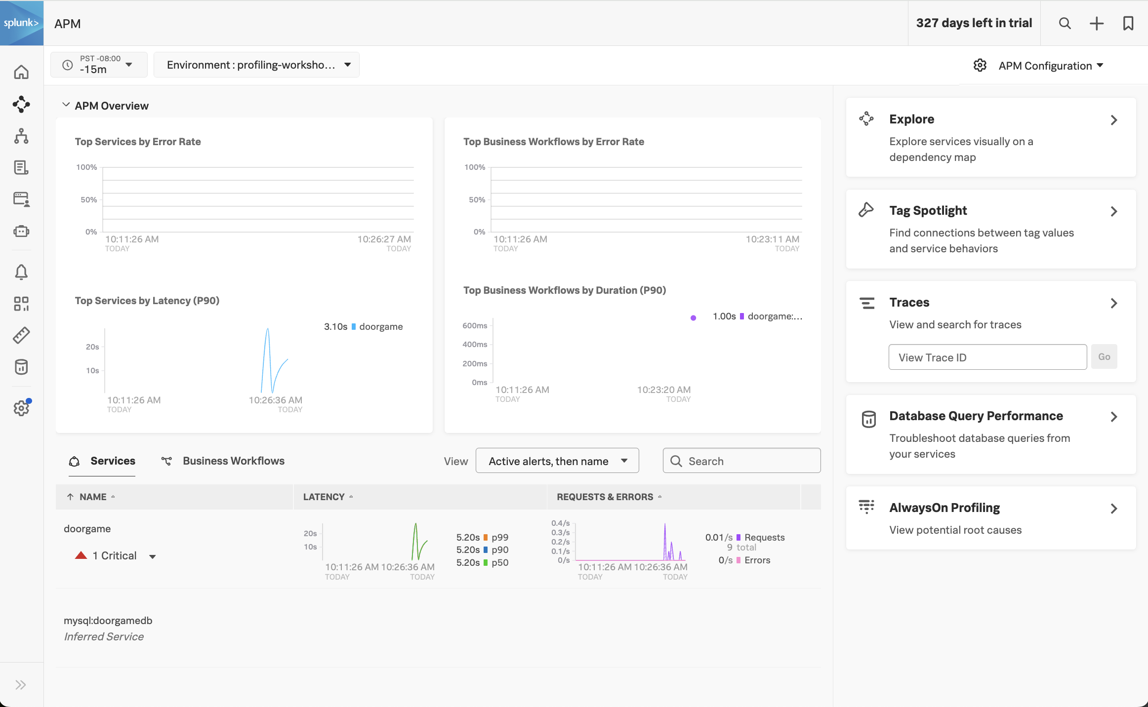
Click on Explore on the right-hand side to view the service map. We should the doorgame application on the service map:
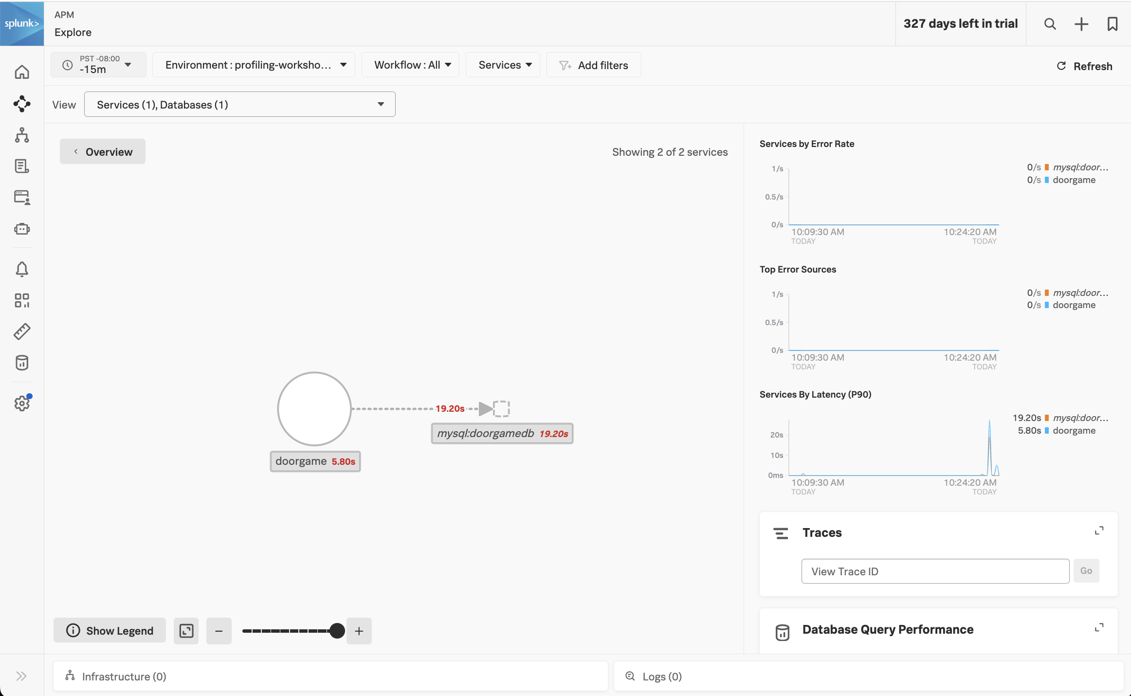
Notice how the majority of the time is being spent in the MySQL database. We can get more details by clicking on Database Query Performance on the right-hand side.

This view shows the SQL queries that took the most amount of time. Ensure that the Compare to dropdown is set to None, so we can focus on current performance.
We can see that one query in particular is taking a long time:
select * from doorgamedb.users, doorgamedb.organizations
(do you notice anything unusual about this query?)
Let’s troubleshoot further by clicking on one of the spikes in the latency graph. This brings up a list of example traces that include this slow query:

Click on one of the traces to see the details:

In the trace, we can see that the DoorGame.startNew operation took 25.8 seconds, and 17.6 seconds of this was associated with the slow SQL query we found earlier.
What did we accomplish?
To recap what we’ve done so far:
- We’ve deployed our application and are able to access it successfully.
- The application is sending traces to Splunk Observability Cloud successfully.
- We started troubleshooting the slow application startup time, and found a slow SQL query that seems to be the root cause.
To troubleshoot further, it would be helpful to get deeper diagnostic data that tells us what’s happening inside our JVM, from both a memory (i.e. JVM heap) and CPU perspective. We’ll tackle that in the next section of the workshop.
Enable AlwaysOn Profiling
20 minutes
Let’s learn how to enable the memory and CPU profilers, verify their operation,
and use the results in Splunk Observability Cloud to find out why our application startup is slow.
Update the application configuration
We will need to pass additional configuration arguments to the Splunk OpenTelemetry Java agent in order to
enable both profilers. The configuration is documented here
in detail, but for now we just need the following settings:
SPLUNK_PROFILER_ENABLED="true"
SPLUNK_PROFILER_MEMORY_ENABLED="true"
Since our application is deployed in Kubernetes, we can update the Kubernetes manifest file to set these environment variables. Open the doorgame/doorgame.yaml file for editing, and ensure the values of the following environment variables are set to “true”:
- name: SPLUNK_PROFILER_ENABLED
  value: "true"
- name: SPLUNK_PROFILER_MEMORY_ENABLED
  value: "true"
Next, let’s redeploy the Door Game application by running the following command:
cd workshop/profiling
kubectl apply -f doorgame/doorgame.yaml
After a few seconds, a new pod will be deployed with the updated application settings.
Confirm operation
To ensure the profiler is enabled, let’s review the application logs with the following commands:
kubectl logs -l app=doorgame --tail=100 | grep JfrActivator
You should see a line in the application log output that shows the profiler is active:
[otel.javaagent 2024-02-05 19:01:12:416 +0000] [main] INFO com.splunk.opentelemetry.profiler.JfrActivator - Profiler is active.```
This confirms that the profiler is enabled and sending data to the OpenTelemetry collector deployed in our Kubernetes cluster, which in turn sends profiling data to Splunk Observability Cloud.
Profiling in APM
Visit http://<your IP address>:81 and play a few more rounds of The Door Game.
Then head back to Splunk Observability Cloud, click on APM, and click on the doorgame service at the bottom of the screen.
Click on “Traces” on the right-hand side to load traces for this service. Filter on traces involving the doorgame service and the GET new-game operation (since we’re troubleshooting the game startup sequence):
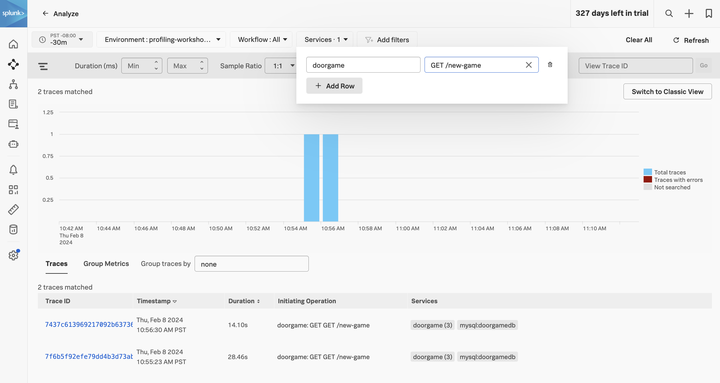
Selecting one of these traces brings up the following screen:

You can see that the spans now include “Call Stacks”, which is a result of us enabling CPU and memory profiling earlier.
Click on the span named doorgame: SELECT doorgamedb, then click on CPU stack traces on the right-hand side:

This brings up the CPU call stacks captured by the profiler.
Let’s open the AlwaysOn Profiler to review the CPU stack trace in more detail. We can do this by clicking on the Span link beside View in AlwaysOn Profiler:
The AlwaysOn Profiler includes both a table and a flamegraph. Take some time to explore this view by doing some of the following:
- click a table item and notice the change in flamegraph
- navigate the flamegraph by clicking on a stack frame to zoom in, and a parent frame to zoom out
- add a search term like
splunk or jetty to highlight some matching stack frames
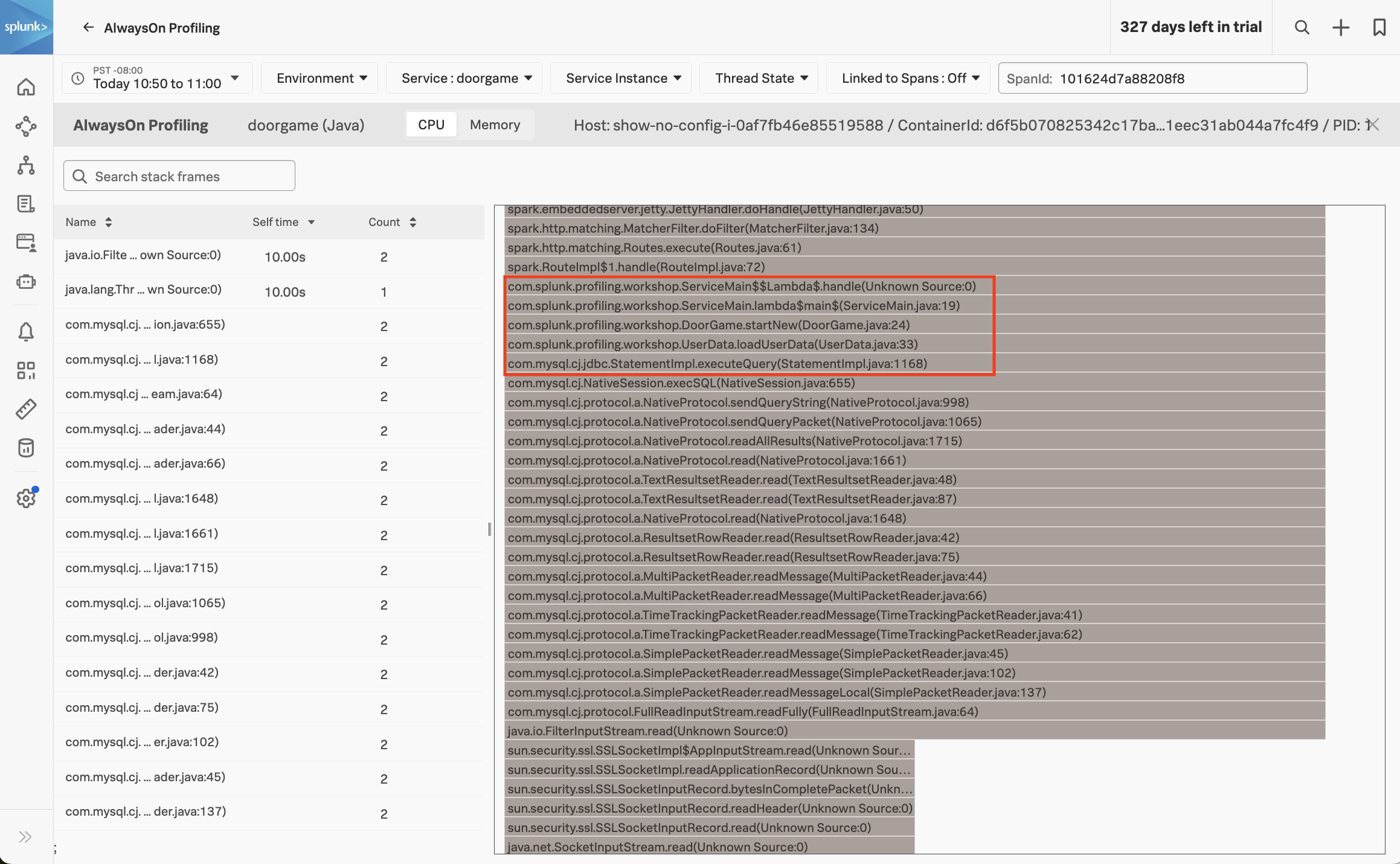
Let’s have a closer look at the stack trace, starting with the DoorGame.startNew method (since we already know that it’s the slowest part of the request)
com.splunk.profiling.workshop.DoorGame.startNew(DoorGame.java:24)
com.splunk.profiling.workshop.UserData.loadUserData(UserData.java:33)
com.mysql.cj.jdbc.StatementImpl.executeQuery(StatementImpl.java:1168)
com.mysql.cj.NativeSession.execSQL(NativeSession.java:655)
com.mysql.cj.protocol.a.NativeProtocol.sendQueryString(NativeProtocol.java:998)
com.mysql.cj.protocol.a.NativeProtocol.sendQueryPacket(NativeProtocol.java:1065)
com.mysql.cj.protocol.a.NativeProtocol.readAllResults(NativeProtocol.java:1715)
com.mysql.cj.protocol.a.NativeProtocol.read(NativeProtocol.java:1661)
com.mysql.cj.protocol.a.TextResultsetReader.read(TextResultsetReader.java:48)
com.mysql.cj.protocol.a.TextResultsetReader.read(TextResultsetReader.java:87)
com.mysql.cj.protocol.a.NativeProtocol.read(NativeProtocol.java:1648)
com.mysql.cj.protocol.a.ResultsetRowReader.read(ResultsetRowReader.java:42)
com.mysql.cj.protocol.a.ResultsetRowReader.read(ResultsetRowReader.java:75)
com.mysql.cj.protocol.a.MultiPacketReader.readMessage(MultiPacketReader.java:44)
com.mysql.cj.protocol.a.MultiPacketReader.readMessage(MultiPacketReader.java:66)
com.mysql.cj.protocol.a.TimeTrackingPacketReader.readMessage(TimeTrackingPacketReader.java:41)
com.mysql.cj.protocol.a.TimeTrackingPacketReader.readMessage(TimeTrackingPacketReader.java:62)
com.mysql.cj.protocol.a.SimplePacketReader.readMessage(SimplePacketReader.java:45)
com.mysql.cj.protocol.a.SimplePacketReader.readMessage(SimplePacketReader.java:102)
com.mysql.cj.protocol.a.SimplePacketReader.readMessageLocal(SimplePacketReader.java:137)
com.mysql.cj.protocol.FullReadInputStream.readFully(FullReadInputStream.java:64)
java.io.FilterInputStream.read(Unknown Source:0)
sun.security.ssl.SSLSocketImpl$AppInputStream.read(Unknown Source:0)
sun.security.ssl.SSLSocketImpl.readApplicationRecord(Unknown Source:0)
sun.security.ssl.SSLSocketInputRecord.bytesInCompletePacket(Unknown Source:0)
sun.security.ssl.SSLSocketInputRecord.readHeader(Unknown Source:0)
sun.security.ssl.SSLSocketInputRecord.read(Unknown Source:0)
java.net.SocketInputStream.read(Unknown Source:0)
java.net.SocketInputStream.read(Unknown Source:0)
java.lang.ThreadLocal.get(Unknown Source:0)
We can interpret the stack trace as follows:
- When starting a new Door Game, a call is made to load user data.
- This results in executing a SQL query to load the user data (which is related to the slow SQL query we saw earlier).
- We then see calls to read data in from the database.
So, what does this all mean? It means that our application startup is slow since it’s spending time loading user data. In fact, the profiler has told us the exact line of code where this happens:
com.splunk.profiling.workshop.UserData.loadUserData(UserData.java:33)
Let’s open the corresponding source file (./doorgame/src/main/java/com/splunk/profiling/workshop/UserData.java) and look at this code in more detail:
public class UserData {

    static final String DB_URL = "jdbc:mysql://mysql/DoorGameDB";
    static final String USER = "root";
    static final String PASS = System.getenv("MYSQL_ROOT_PASSWORD");
    static final String SELECT_QUERY = "select * FROM DoorGameDB.Users, DoorGameDB.Organizations";

    HashMap<String, User> users;

    public UserData() {
        users = new HashMap<String, User>();
    }

    public void loadUserData() {

        // Load user data from the database and store it in a map
        Connection conn = null;
        Statement stmt = null;
        ResultSet rs = null;

        try{
            conn = DriverManager.getConnection(DB_URL, USER, PASS);
            stmt = conn.createStatement();
            rs = stmt.executeQuery(SELECT_QUERY);
            while (rs.next()) {
                User user = new User(rs.getString("UserId"), rs.getString("FirstName"), rs.getString("LastName"));
                users.put(rs.getString("UserId"), user);
            }
Here we can see the application logic in action. It establishes a connection to the database, then executes the SQL query we saw earlier:
select * FROM DoorGameDB.Users, DoorGameDB.Organizations
It then loops through each of the results, and loads each user into a HashMap object, which is a collection of User objects.
We have a good understanding of why the game startup sequence is so slow, but how do we fix it?
For more clues, let’s have a look at the other part of AlwaysOn Profiling: memory profiling. To do this, click on the Memory tab in AlwaysOn profiling:
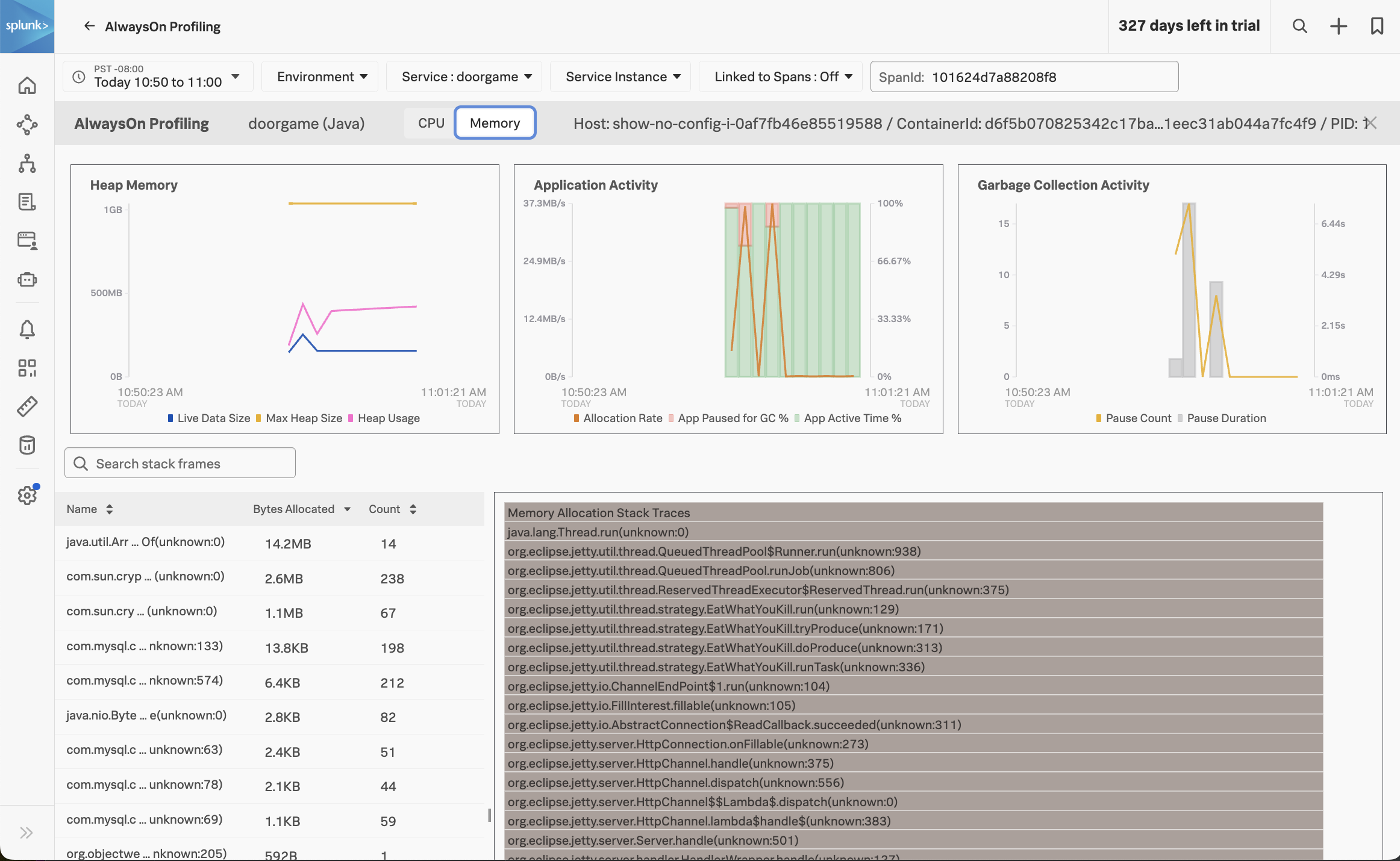
At the top of this view, we can see how much heap memory our application is using, the heap memory allocation rate, and garbage collection activity.
We can see that our application is using about 400 MB out of the max 1 GB heap size, which seems excessive for such a simple application. We can also see that some garbage collection occurred, which caused our application to pause (and probably annoyed those wanting to play the Game Door).
At the bottom of the screen, which can see which methods in our Java application code are associated with the most heap memory usage. Click on the first item in the list to show the Memory Allocation Stack Traces associated with the java.util.Arrays.copyOf method specifically:

With help from the profiler, we can see that the loadUserData method not only consumes excessive CPU time, but it also consumes excessive memory when storing the user data in the HashMap collection object.
What did we accomplish?
We’ve come a long way already!
- We learned how to enable the profiler in the Splunk OpenTelemetry Java instrumentation agent.
- We learned how to verify in the agent output that the profiler is enabled.
- We have explored several profiling related workflows in APM:
- How to navigate to AlwaysOn Profiling from the troubleshooting view
- How to explore the flamegraph and method call duration table through navigation and filtering
- How to identify when a span has sampled call stacks associated with it
- How to explore heap utilization and garbage collection activity
- How to view memory allocation stack traces for a particular method
In the next section, we’ll apply a fix to our application to resolve the slow startup performance.
Fix Application Startup Slowness
10 minutes
In this section, we’ll use what we learned from the profiling data in Splunk Observability Cloud to resolve the slowness we saw when starting our application.
Examining the Source Code
Open the corresponding source file once again (./doorgame/src/main/java/com/splunk/profiling/workshop/UserData.java) and focus on the following code:
public class UserData {

    static final String DB_URL = "jdbc:mysql://mysql/DoorGameDB";
    static final String USER = "root";
    static final String PASS = System.getenv("MYSQL_ROOT_PASSWORD");
    static final String SELECT_QUERY = "select * FROM DoorGameDB.Users, DoorGameDB.Organizations";

    HashMap<String, User> users;

    public UserData() {
        users = new HashMap<String, User>();
    }

    public void loadUserData() {

        // Load user data from the database and store it in a map
        Connection conn = null;
        Statement stmt = null;
        ResultSet rs = null;

        try{
            conn = DriverManager.getConnection(DB_URL, USER, PASS);
            stmt = conn.createStatement();
            rs = stmt.executeQuery(SELECT_QUERY);
            while (rs.next()) {
                User user = new User(rs.getString("UserId"), rs.getString("FirstName"), rs.getString("LastName"));
                users.put(rs.getString("UserId"), user);
            }
After speaking with a database engineer, you discover that the SQL query being executed includes a cartesian join:
select * FROM DoorGameDB.Users, DoorGameDB.Organizations
Cartesian joins are notoriously slow, and shouldn’t be used, in general.
Upon further investigation, you discover that there are 10,000 rows in the user table, and 1,000 rows in the organization table. When we execute a cartesian join using both of these tables, we end up with 10,000 x 1,000 rows being returned, which is 10,000,000 rows!
Furthermore, the query ends up returning duplicate user data, since each record in the user table is repeated for each organization.
So when our code executes this query, it tries to load 10,000,000 user objects into the HashMap, which explains why it takes so long to execute, and why it consumes so much heap memory.
Let’s Fix That Bug
After consulting the engineer that originally wrote this code, we determined that the join with the Organizations table was inadvertent.
So when loading the users into the HashMap, we simply need to remove this table from the query.
Open the corresponding source file once again (./doorgame/src/main/java/com/splunk/profiling/workshop/UserData.java) and change the following line of code:
static final String SELECT_QUERY = "select * FROM DoorGameDB.Users, DoorGameDB.Organizations";
to:
static final String SELECT_QUERY = "select * FROM DoorGameDB.Users";
Now the method should perform much more quickly, and less memory should be used, as it’s loading the correct number of users into the HashMap (10,000 instead of 10,000,000).
Rebuild and Redeploy Application
Let’s test our changes by using the following commands to re-build and re-deploy the Door Game application:
cd workshop/profiling
./5-redeploy-doorgame.sh
Once the application has been redeployed successfully, visit The Door Game again to confirm that your fix is in place:
http://<your IP address>:81
Clicking Let's Play should take us to the game more quickly now (though performance could still be improved):

Start the game a few more times, then return to Splunk Observability Cloud to confirm that the latency of the GET new-game operation has decreased.
What did we accomplish?
- We discovered why our SQL query was so slow.
- We applied a fix, then rebuilt and redeployed our application.
- We confirmed that the application starts a new game more quickly.
In the next section, we’ll explore continue playing the game and fix any remaining performance issues that we find.
Fix In Game Slowness
10 minutes
Now that our game startup slowness has been resolved, let’s play several rounds of the Door Game and ensure the rest of the game performs quickly.
As you play the game, do you notice any other slowness? Let’s look at the data in Splunk Observability Cloud to put some numbers on what we’re seeing.
Navigate to APM then click on Traces on the right-hand side of the screen. Sort the traces by Duration in descending order:
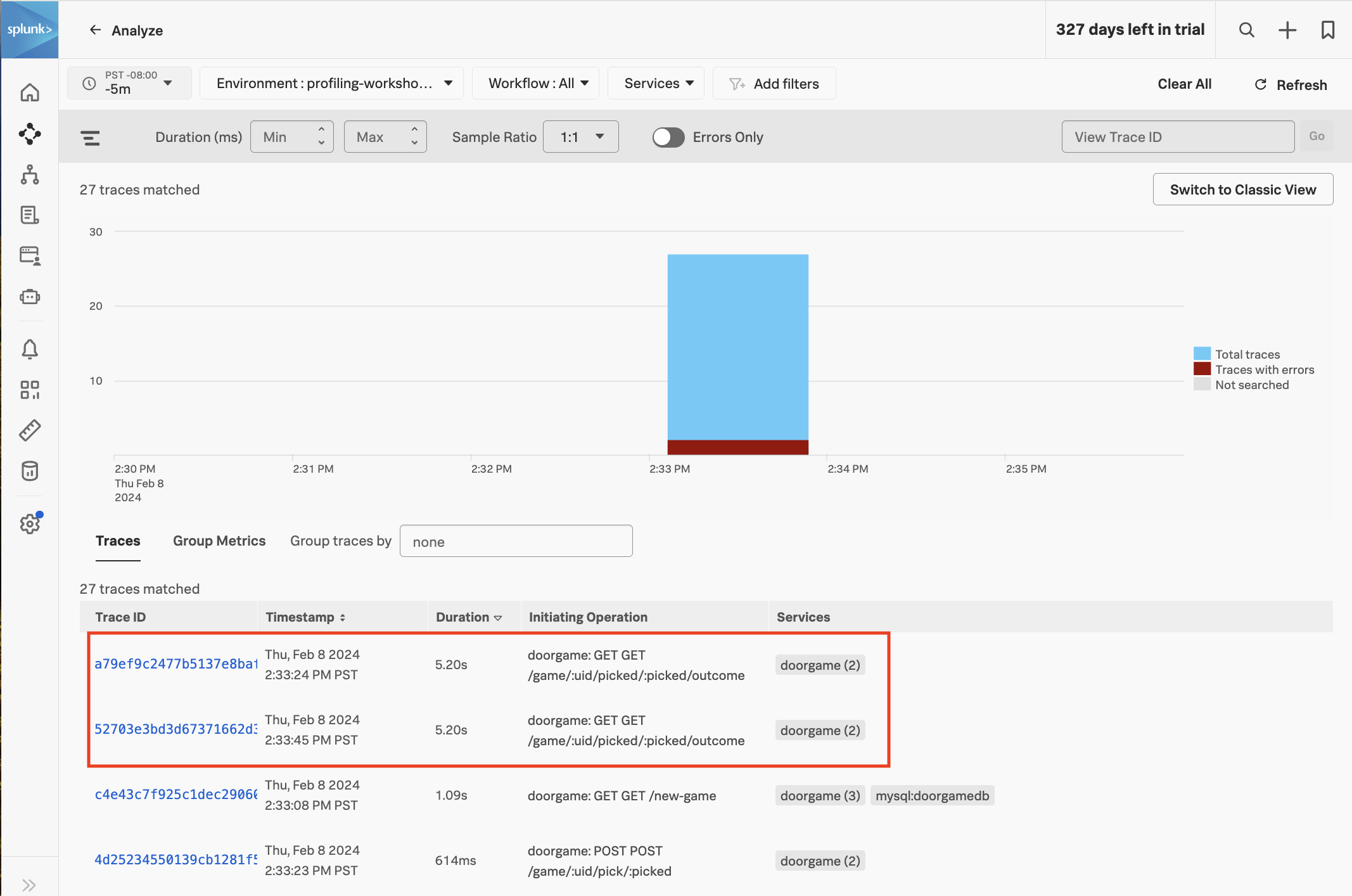
We can see that a few of the traces with an operation of GET /game/:uid/picked/:picked/outcome have a duration of just over five seconds. This explains why we’re still seeing some slowness when we play the app (note that the slowness is no longer on the game startup operation, GET /new-game, but rather a different operation used while actually playing the game).
Let’s click on one of the slow traces and take a closer look. Since profiling is still enabled, call stacks have been captured as part of this trace. Click on the child span in the waterfall view, then click CPU Stack Traces:

At the bottom of the call stack, we can see that the thread was busy sleeping:
com.splunk.profiling.workshop.ServiceMain$$Lambda$.handle(Unknown Source:0)
com.splunk.profiling.workshop.ServiceMain.lambda$main$(ServiceMain.java:34)
com.splunk.profiling.workshop.DoorGame.getOutcome(DoorGame.java:41)
com.splunk.profiling.workshop.DoorChecker.isWinner(DoorChecker.java:14)
com.splunk.profiling.workshop.DoorChecker.checkDoorTwo(DoorChecker.java:30)
com.splunk.profiling.workshop.DoorChecker.precheck(DoorChecker.java:36)
com.splunk.profiling.workshop.Util.sleep(Util.java:9)
java.util.concurrent.TimeUnit.sleep(Unknown Source:0)
java.lang.Thread.sleep(Unknown Source:0)
java.lang.Thread.sleep(Native Method:0)
The call stack tells us a story – reading from the bottom up, it lets us describe
what is happening inside the service code. A developer, even one unfamiliar with the
source code, should be able to look at this call stack to craft a narrative like:
We are getting the outcome of a game. We leverage the DoorChecker to
see if something is the winner, but the check for door two somehow issues
a precheck() that, for some reason, is deciding to sleep for a long time.
Our workshop application is left intentionally simple – a real-world service might see the
thread being sampled during a database call or calling into an un-traced external service.
It is also possible that a slow span is executing a complicated business process,
in which case maybe none of the stack traces relate to each other at all.
The longer a method or process is, the greater chance we will have call stacks
sampled during its execution.
Let’s Fix That Bug
By using the profiling tool, we were able to determine that our application is slow
when issuing the DoorChecker.precheck() method from inside DoorChecker.checkDoorTwo().
Let’s open the doorgame/src/main/java/com/splunk/profiling/workshop/DoorChecker.java source file in our editor.
By quickly glancing through the file, we see that there are methods for checking
each door, and all of them call precheck(). In a real service, we might be uncomfortable
simply removing the precheck() call because there could be unseen/unaccounted side
effects.
Down on line 29 we see the following:
    private boolean checkDoorTwo(GameInfo gameInfo) {
        precheck(2);
        return gameInfo.isWinner(2);
    }

    private void precheck(int doorNum) {
        long extra = (int)Math.pow(70, doorNum);
        sleep(300 + extra);
    }
With our developer hat on, we notice that the door number is zero based, so
the first door is 0, the second is 1, and the 3rd is 2 (this is conventional).
The extra value is used as extra/additional sleep time, and it is computed by taking
70^doorNum (Math.pow performs an exponent calculation). That’s odd, because this means:
- door 0 => 70^0 => 1ms
- door 1 => 70^1 => 70ms
- door 2 => 70^2 => 4900ms
We’ve found the root cause of our slow bug! This also explains why the first two doors
weren’t ever very slow.
We have a quick chat with our product manager and team lead, and we agree that the precheck()
method must stay but that the extra padding isn’t required. Let’s remove the extra variable
and make precheck now read like this:
    private void precheck(int doorNum) {
        sleep(300);
    }
Now all doors will have a consistent behavior. Save your work and then rebuild and redeploy the application using the following command:
cd workshop/profiling
./5-redeploy-doorgame.sh
Once the application has been redeployed successfully, visit The Door Game again to confirm that your fix is in place:
http://<your IP address>:81
What did we accomplish?
- We found another performance issue with our application that impacts game play.
- We used the CPU call stacks included in the trace to understand application behavior.
- We learned how the call stack can tell us a story and point us to suspect lines of code.
- We identified the slow code and fixed it to make it faster.
Summary
3 minutes
In this workshop, we accomplished the following:
- We deployed our application and captured traces with Splunk Observability Cloud.
- We used Database Query Performance to find a slow-running query that impacted the game startup time.
- We enabled AlwaysOn Profiling and used it to confirm which line of code was causing the increased startup time and memory usage.
- We found another application performance issue and used AlwaysOn Profiling again to find the problematic line of code.
- We applied fixes for both of these issues and verified the result using Splunk Observability Cloud.
Enabling AlwaysOn Profiling and utilizing Database Query Performance for your applications will let you get even more value from the data you’re sending to Splunk Observability Cloud.
Now that you’ve completed this workshop, you have the knowledge you need to start collecting deeper diagnostic data from your own applications!
To get started with Database Query Performance today, check out Monitor Database Query Performance.
And to get started with AlwaysOn Profiling, check out Introduction to AlwaysOn Profiling for Splunk APM
For more help, feel free to ask a Splunk Expert.