Working with Dashboards
20 minutes
- Introduction to the Dashboards and Charts
- Editing and creating charts
- Filtering and analytical functions
- Using formulas
- Saving charts in a dashboard
- Introduction to SignalFlow
1. Dashboards
Dashboards are groupings of charts and visualizations of metrics. Well-designed dashboards can provide useful and actionable insight into your system at a glance. Dashboards can be complex or contain just a few charts that drill down only into the data you want to see.
During this module, we are going to create the following charts and dashboard and connect them to your Team page.
2. Your Teams’ Page
Click on the  from the navbar. As you have already been assigned to a team, you will land on the team dashboard. We use the Example Team as an example here. The one in your workshop will be different!
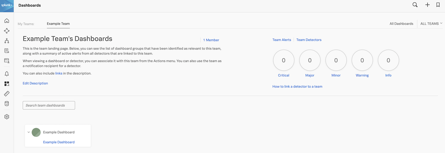
This page shows the total number of team members, how many active alerts for your team and all dashboards that are assigned to your team. Right now there are no dashboards assigned but as stated before, we will add the new dashboard that you will create to your Teams page later.
3. Sample Charts
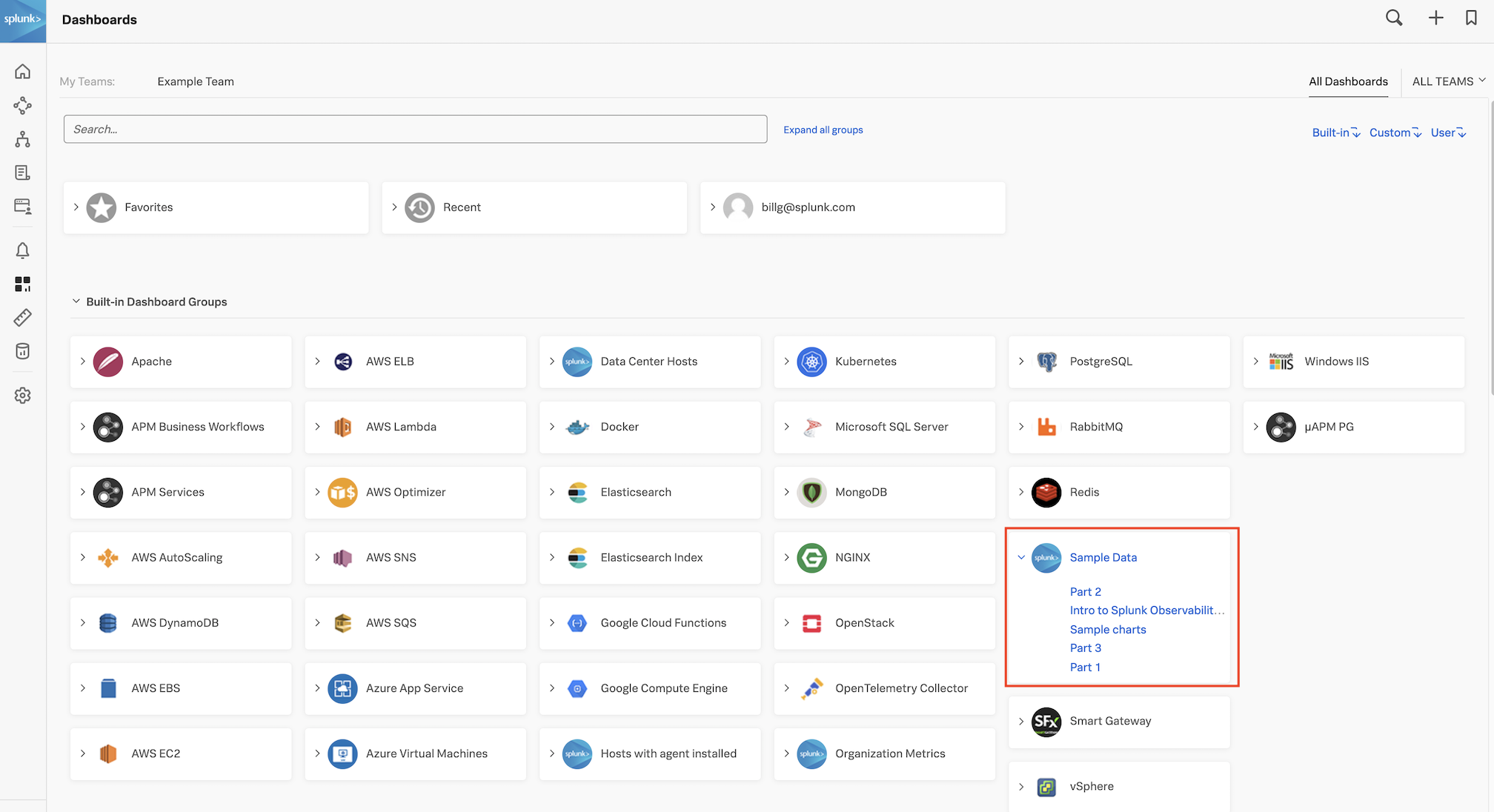
To continue, click on All Dashboards in the top right corner of the screen. This brings you to the view that shows all the available dashboards, including the pre-built ones.
If you are already receiving metrics from a Cloud API integration or another service through the Splunk Agent you will see relevant dashboards for these services.
4. Inspecting the Sample Data
Among the dashboards, you will see a Dashboard group called Sample Data. Expand the Sample Data dashboard group by clicking on it, and then click on the Sample Charts dashboard.
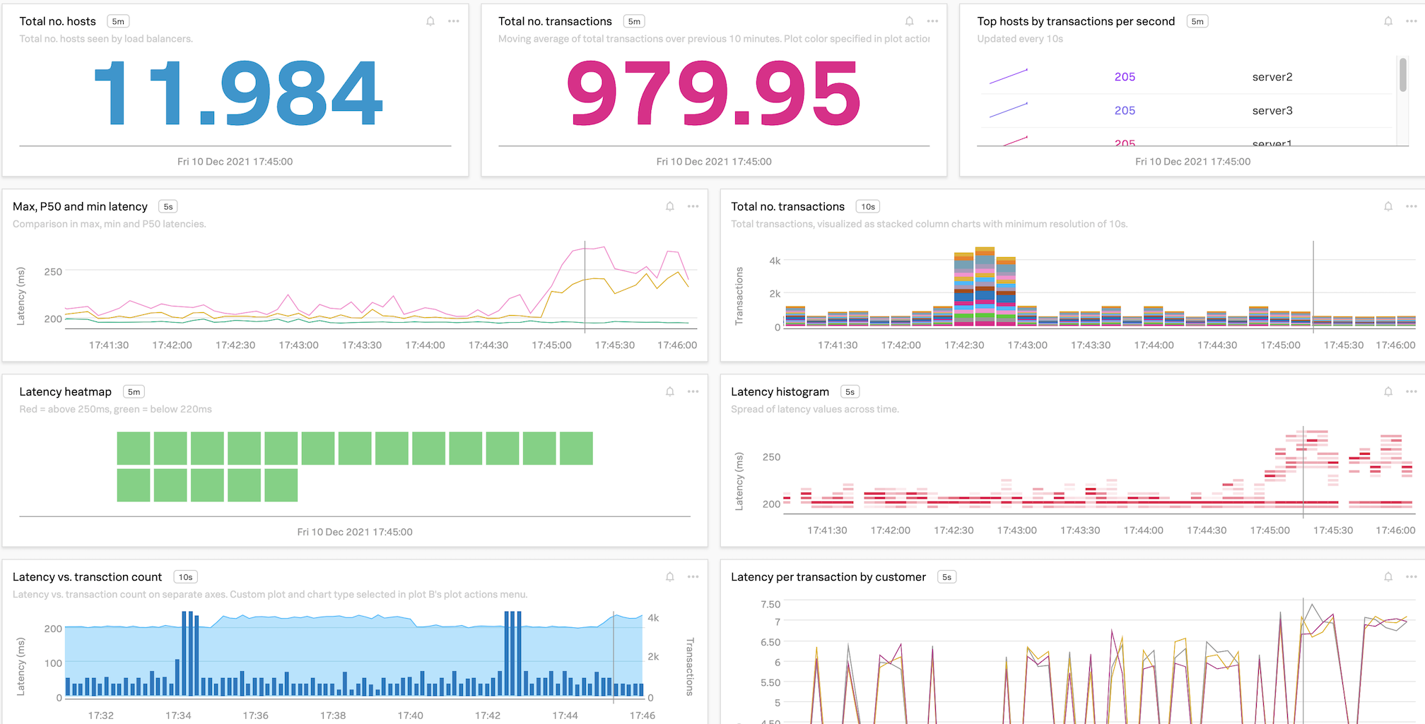
In the Sample Charts dashboard, you can see a selection of charts that show a sample of the various styles, colors and formats you can apply to your charts in the dashboards.
Have a look through all the dashboards in this dashboard group (PART 1, PART 2, PART 3 and INTRO TO SPLUNK OBSERVABILITY CLOUD)
Subsections of Working with Dashboards
Editing charts
1. Editing a chart
Select the SAMPLE CHARTS dashboard and then click on the three dots ... on the Latency histogram chart, then on Open (or you can click on the name of the chart which here is Latency histogram).
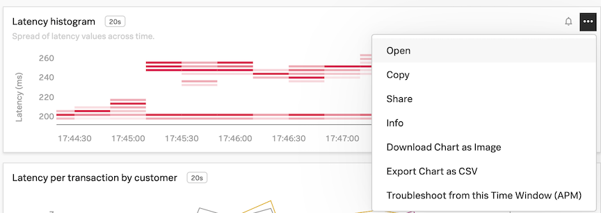
You will see the plot options, current plot and signal (metric) for the Latency histogram chart in the chart editor UI.

In the Plot Editor tab under Signal you see the metric demo.trans.latency we are currently plotting.
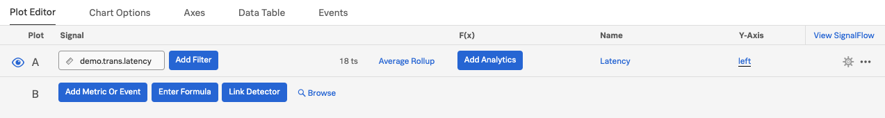
You will see a number of Line plots. The number 18 ts indicates that we are plotting 18 metric time series in the chart.
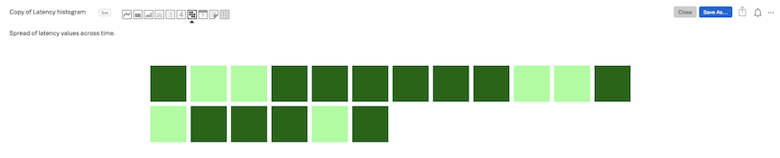
Click on the different chart type icons to explore each of the visualizations. Notice their name while you swipe over them. For example, click on the Heat Map icon:

See how the chart changes to a heat map.
Note
You can use different charts to visualize your metrics - you choose which chart type fits best for the visualization you want to have.
For more info on the different chart types see Choosing a chart type.
Click on the Line chart type and you will see the line plot.
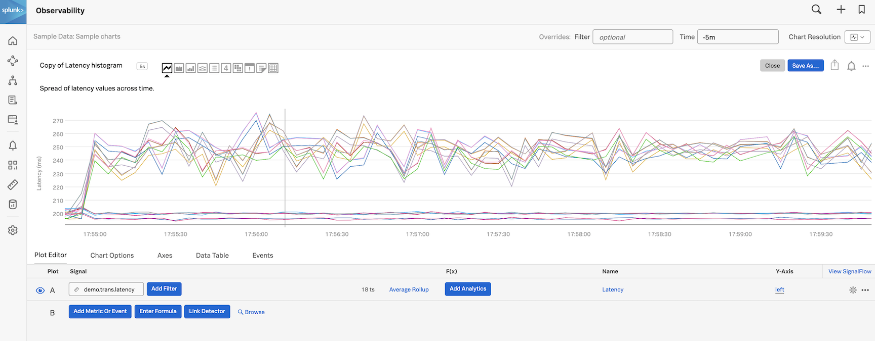
2. Changing the time window
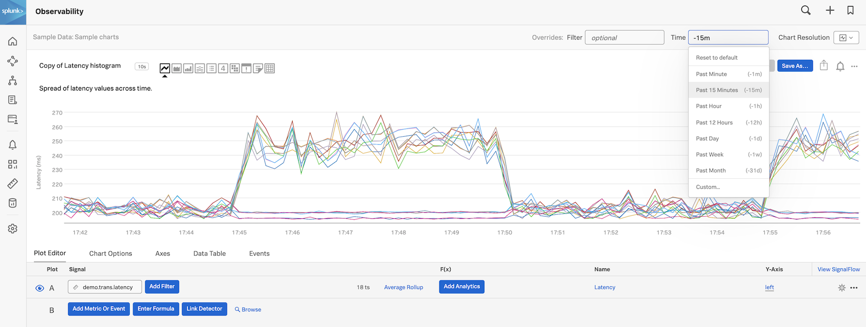
You can also increase the time window of the chart by changing the time to Past 15 minutes by selecting from the Time dropdown.
3. Viewing the Data Table
Click on the Data Table tab.
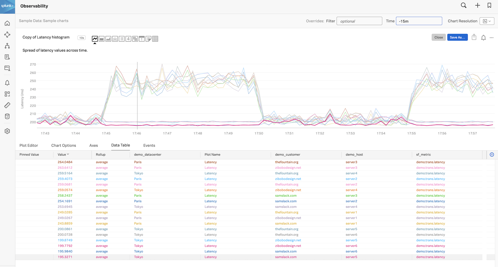
You now see 18 rows, each representing a metric time series with a number of columns. These columns represent the dimensions of the metric. The dimensions for demo.trans.latency are:
demo_datacenterdemo_customerdemo_host
In the demo_datacenter column you see that there are two data centers, Paris and Tokyo, for which we are getting metrics.
If you move your cursor over the lines in the chart horizontally you will see the data table update accordingly. If you click on one of the lines in the chart you will see a pinned value appear in the data table.
Now click on Plot editor again to close the Data Table and let’s save this chart into a dashboard for later use!
Saving charts
1. Saving a chart
To start saving your chart, lets give it a name and description. Click the name of the chart Copy of Latency Histogram and rename it to “Active Latency”.
To change the description click on Spread of latency values across time. and change this to Overview of latency values in real-time.
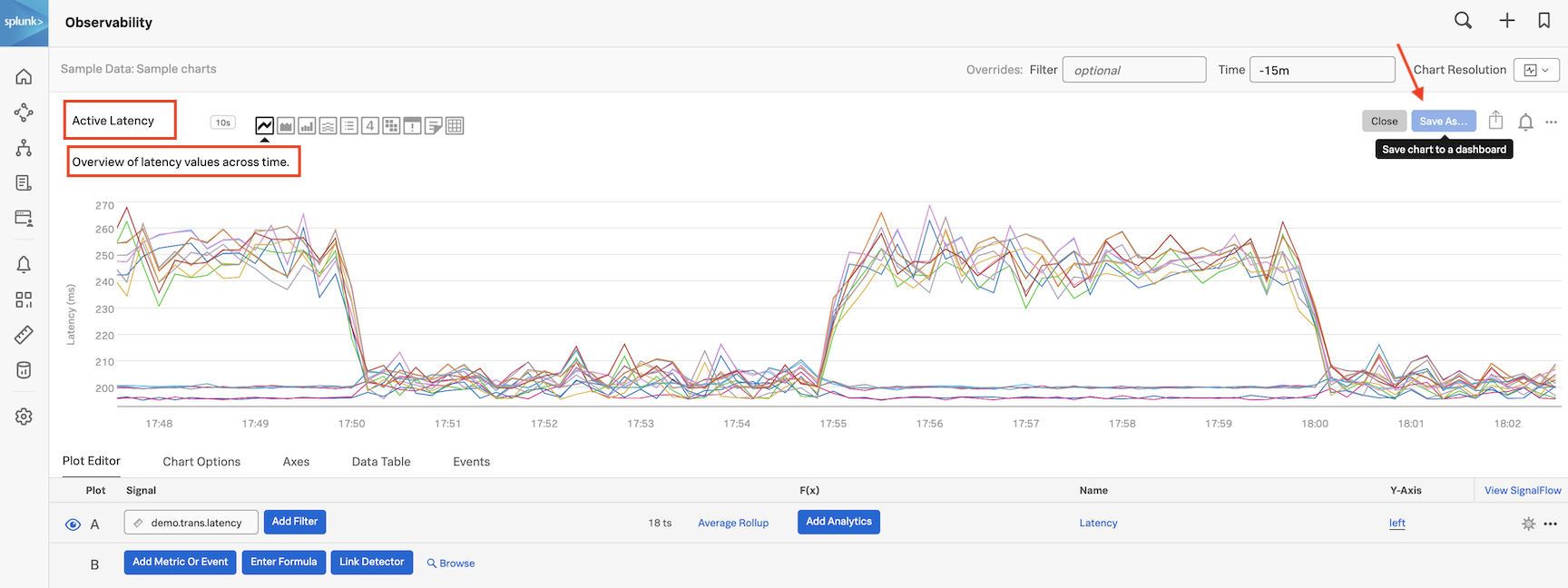
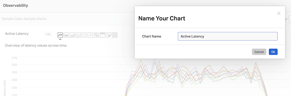
Click the Save As button. Make sure your chart has a name, it will use the name Active Latency the you defined in the previous step, but you can edit it here if needed.
Press the Ok
button to continue.
2. Creating a dashboard
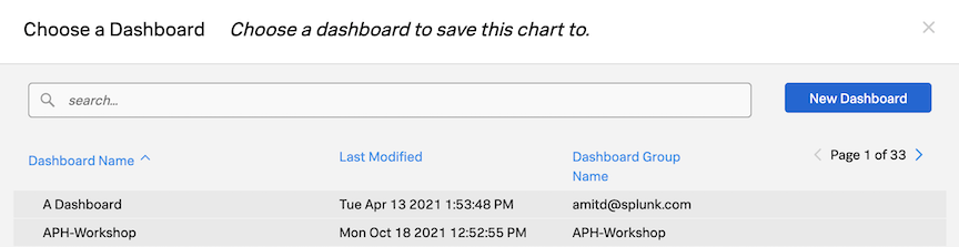
In the Choose dashboard dialog, we need to create a new dashboard, click on the New Dashboard
button.
You will now see the New Dashboard Dialog. In here you can give you dashboard a name and description, and set Read and Write Permissions.
Please use your own name in the following format to give your dashboard a name e.g. YOUR_NAME-Dashboard.
Please replace YOUR_NAME with your own name, change the dashboard permissions to Restricted Read and Write access, and verify your user can read/write.
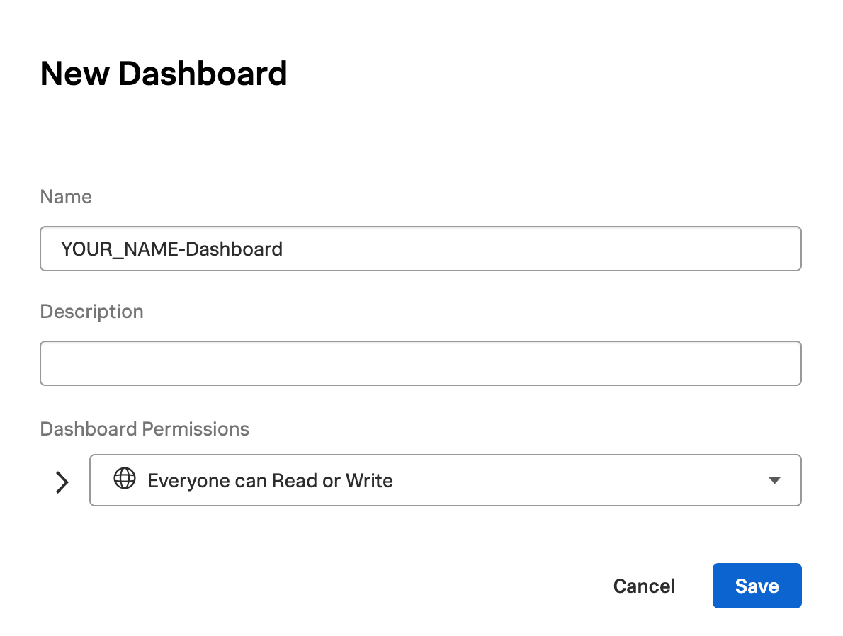
You should see you own login information displayed, meaning you are now the only one who can edit this dashboard. Of course you have the option to add other users or teams from the drop box below that may edit your dashboard and charts, but for now make sure you change it back to Everyone can Read or Write to remove any restrictions and press the Save
Button to continue.
Your new dashboard is now available and selected so you can save your chart in your new dashboard.
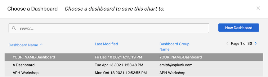
Make sure you have your dashboard selected and press the Ok button.
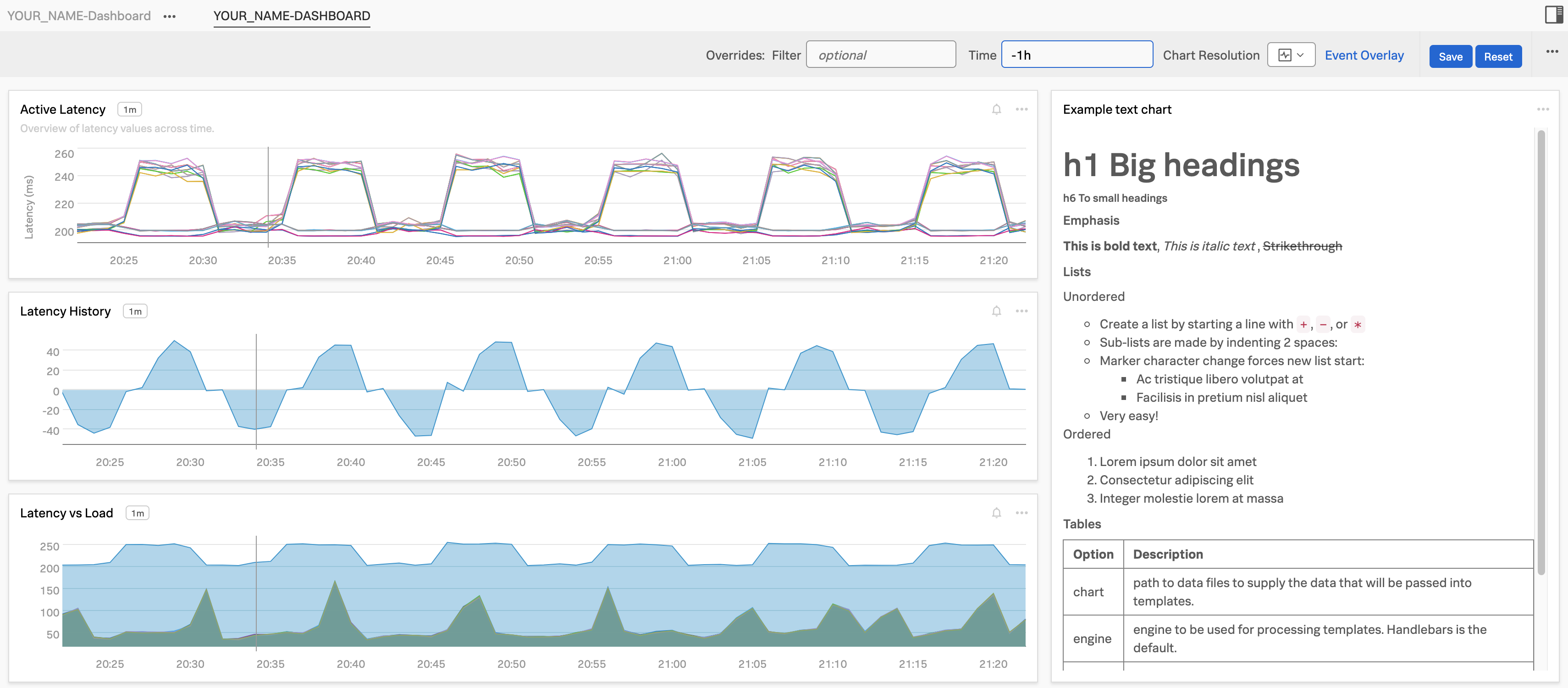
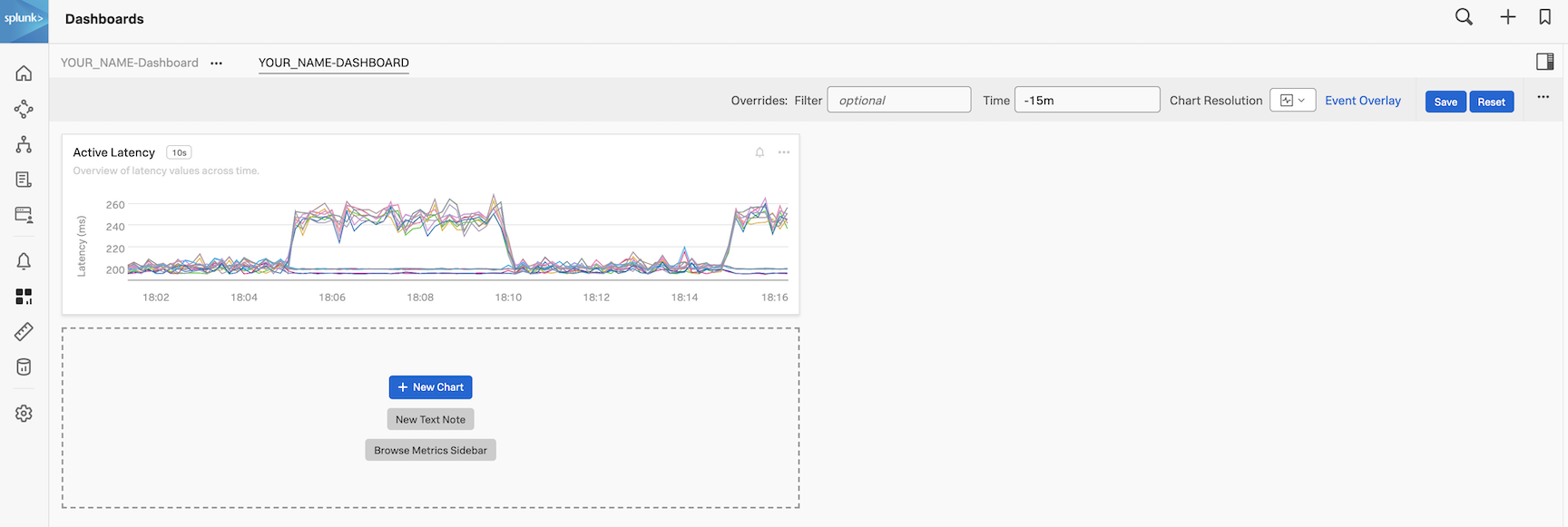
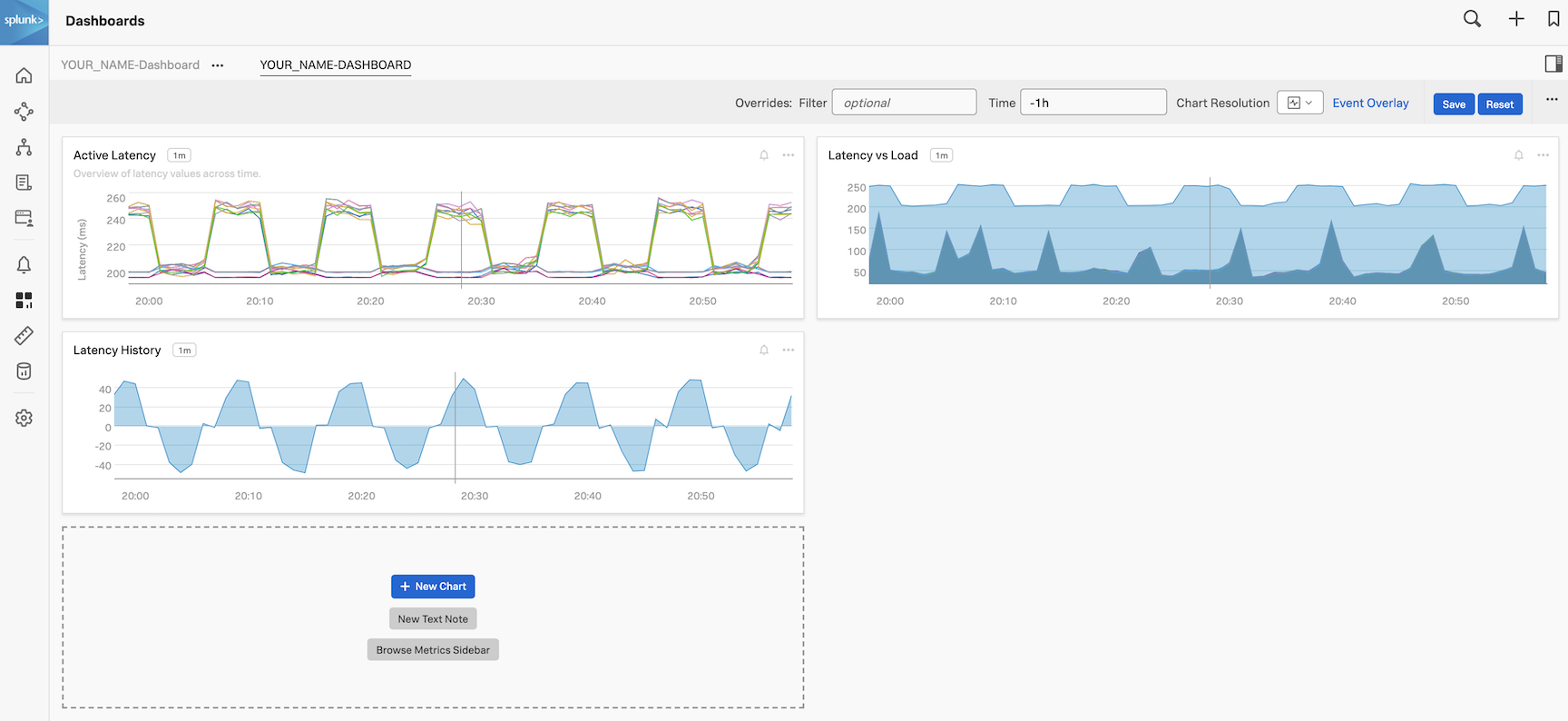
You will now be taken to your dashboard like below. You can see at the top left that your YOUR_NAME-DASHBOARD is part of a Dashboard Group YOUR_NAME-Dashboard. You can add other dashboards to this dashboard group.
3. Add to Team page
It is common practice to link dashboards that are relevant to a Team to a teams page. So let’s add your dashboard to the team page for easy access later. Use the  from the navbar again.
This will bring you to your teams dashboard, We use the team Example Team as an example here, the workshop one will be different.

Press the + Add Dashboard Group button to add you dashboard to the team page.
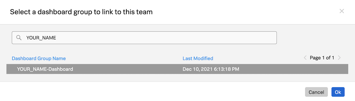
This will bring you to the Select a dashboard group to link to this team dialog.
Type your name (that you used above) in the search box to find your Dashboard. Select it so its highlighted and click the Ok button to add your dashboard.
Your dashboard group will appear as part of the team page. Please note during the course of the workshop many more will appear here.
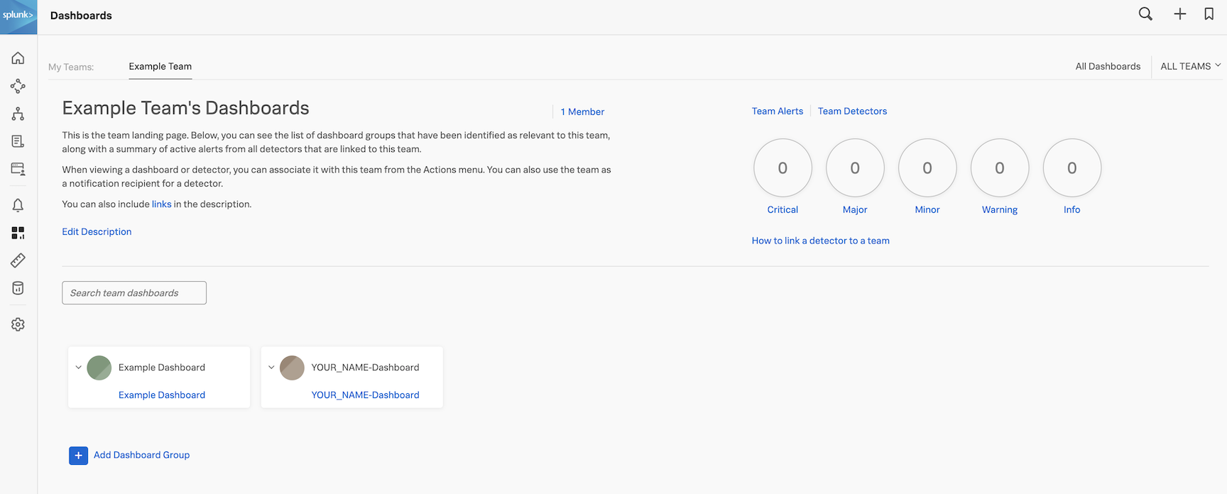
Now click on the link for your Dashboard to add more charts!
1 Creating a new chart
Let’s now create a new chart and save it in our dashboard!
Select the plus icon (top right of the UI) and from the drop down, choose the option Chart.
Or click on the + New Chart Button to create a new chart.

You will now see a chart template like the following.
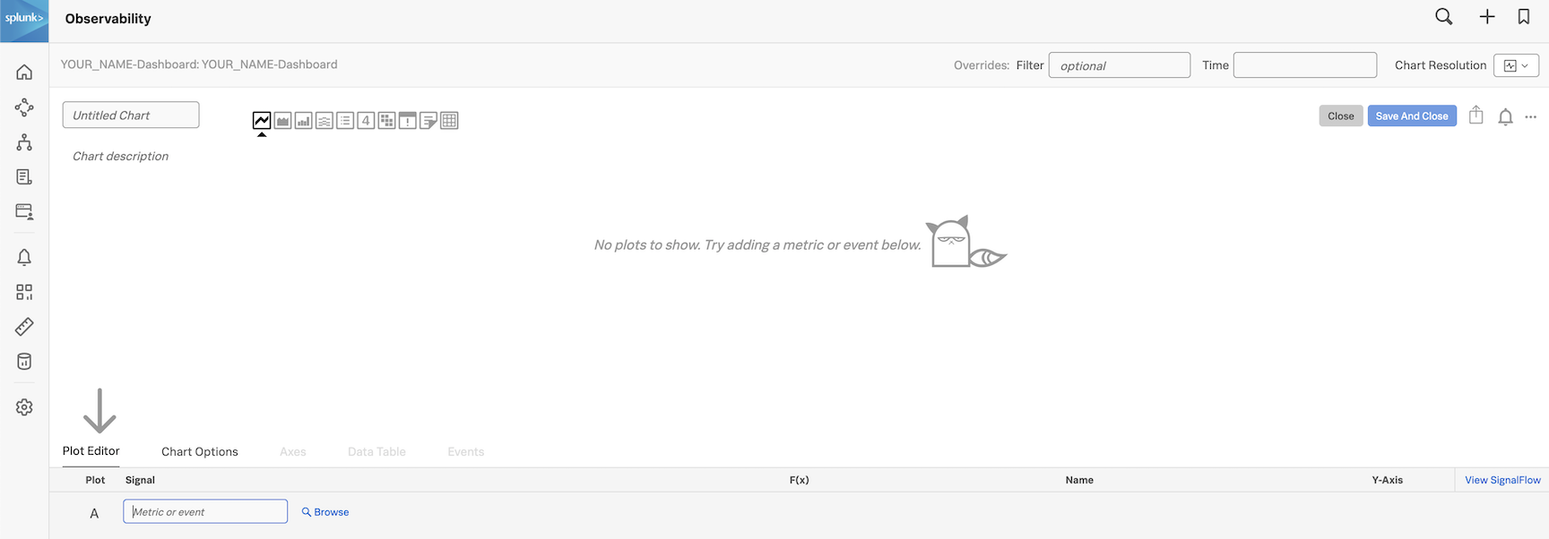
Let’s enter a metric to plot. We are still going to use the metric demo.trans.latency.
In the Plot Editor tab under Signal enter demo.trans.latency.

You should now have a familiar line chart. Please switch the time to 15 mins.

2. Filtering and Analytics
Let’s now select the Paris datacenter to do some analytics - for that we will use a filter.
Let’s go back to the Plot Editor tab and click on Add Filter
, wait until it automatically populates, choose demo_datacenter, and then Paris.

In the F(x) column, add the analytic function Percentile:Aggregation, and leave the value to 95 (click outside to confirm).

For info on the Percentile function and the other functions see Chart Analytics.
3. Using Timeshift analytical function
Let’s now compare with older metrics. Click on ... and then on Clone in the dropdown to clone Signal A.

You will see a new row identical to A, called B, both visible and plotted.

For Signal B, in the F(x) column add the analytic function Timeshift and enter 1w (or 7d for 7 days), and click outside to confirm.

Click on the cog on the far right, and choose a Plot Color e.g. pink, to change color for the plot of B.

Click on Close.
We now see plots for Signal A (the past 15 minutes) as a blue plot, and the plots from a week ago in pink.
In order to make this clearer we can click on the Area chart icon to change the visualization.

We now can see when last weeks latency was higher!
Next, click into the field next to Time on the Override bar and choose Past Hour from the dropdown.

Let’s now plot the difference of all metric values for a day with 7 days in between.
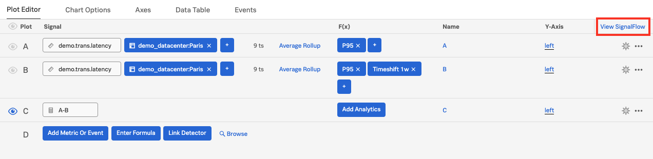
Click on Enter Formula
then enter A-B (A minus B) and hide (deselect) all Signals using the eye, except C.

We now see only the difference of all metric values of A and B being plotted. We see that we have some negative values on the plot because a metric value of B has some times larger value than the metric value of A at that time.
Lets look at the Signalflow that drives our Charts and Detectors!
3.4 SignalFlow
1. Introduction
Let’s take a look at SignalFlow - the analytics language of Observability Cloud that can be used to setup monitoring as code.
The heart of Splunk Infrastructure Monitoring is the SignalFlow analytics engine that runs computations written in a Python-like language. SignalFlow programs accept streaming input and produce output in real time. SignalFlow provides built-in analytical functions that take metric time series (MTS) as input, perform computations, and output a resulting MTS.
- Comparisons with historical norms, e.g. on a week-over-week basis
- Population overviews using a distributed percentile chart
- Detecting if the rate of change (or other metric expressed as a ratio, such as a service level objective) has exceeded a critical threshold
- Finding correlated dimensions, e.g. to determine which service is most correlated with alerts for low disk space
Infrastructure Monitoring creates these computations in the Chart Builder user interface, which lets you specify the input MTS to use and the analytical functions you want to apply to them. You can also run SignalFlow programs directly by using the SignalFlow API.
SignalFlow includes a large library of built-in analytical functions that take a metric time series as an input, performs computations on its datapoints, and outputs time series that are the result of the computation.
2. View SignalFlow
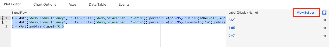
In the chart builder, click on View SignalFlow.
You will see the SignalFlow code that composes the chart we were working on. You can now edit the SignalFlow directly within the UI. Our documentation has the full list of SignalFlow functions and methods.
Also, you can copy the SignalFlow and use it when interacting with the API or with Terraform to enable Monitoring as Code.
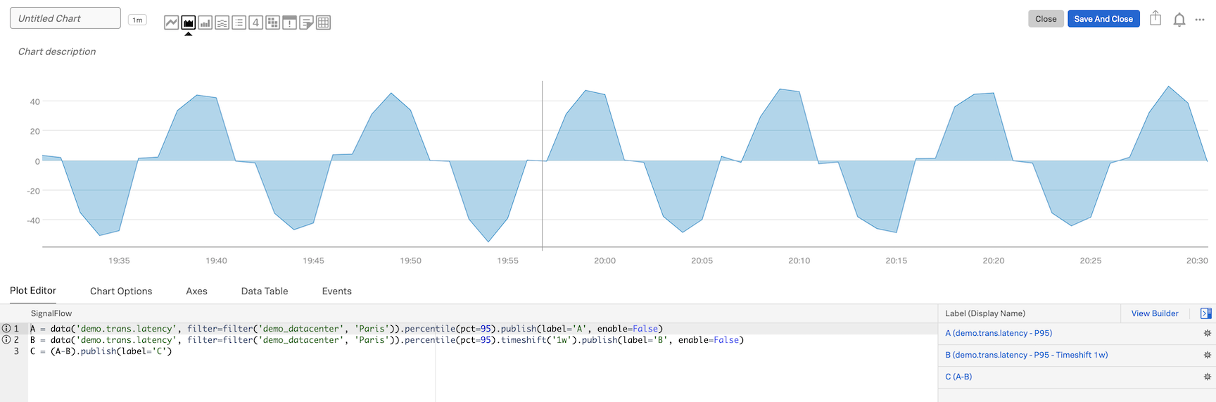
A = data('demo.trans.latency', filter=filter('demo_datacenter', 'Paris')).percentile(pct=95).publish(label='A', enable=False)
B = data('demo.trans.latency', filter=filter('demo_datacenter', 'Paris')).percentile(pct=95).timeshift('1w').publish(label='B', enable=False)
C = (A-B).publish(label='C')
Click on View Builder to go back to the Chart Builder UI.
Let’s save this new chart to our Dashboard!
Adding charts to dashboards
1. Save to existing dashboard
Check that you have YOUR_NAME-Dashboard: YOUR_NAME-Dashboard in the top left corner. This means you chart will be saved in this Dashboard.
Name the Chart Latency History and add a Chart Description if you wish.
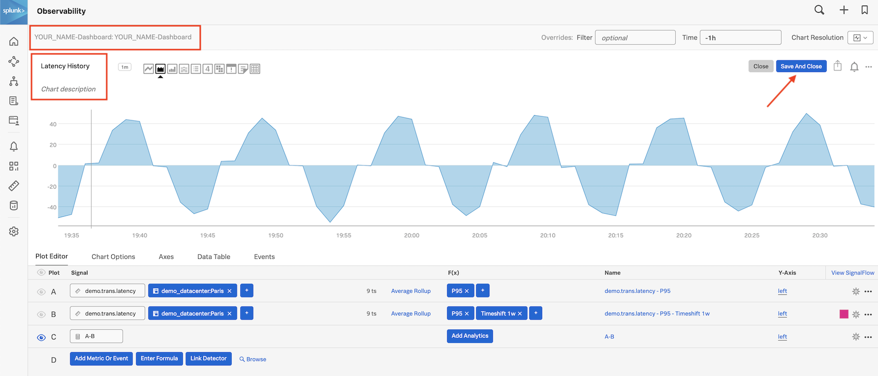
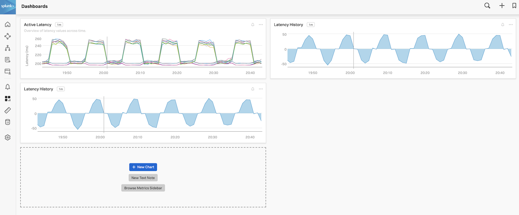
Click on Save And Close. This returns you to your dashboard that now has two charts!
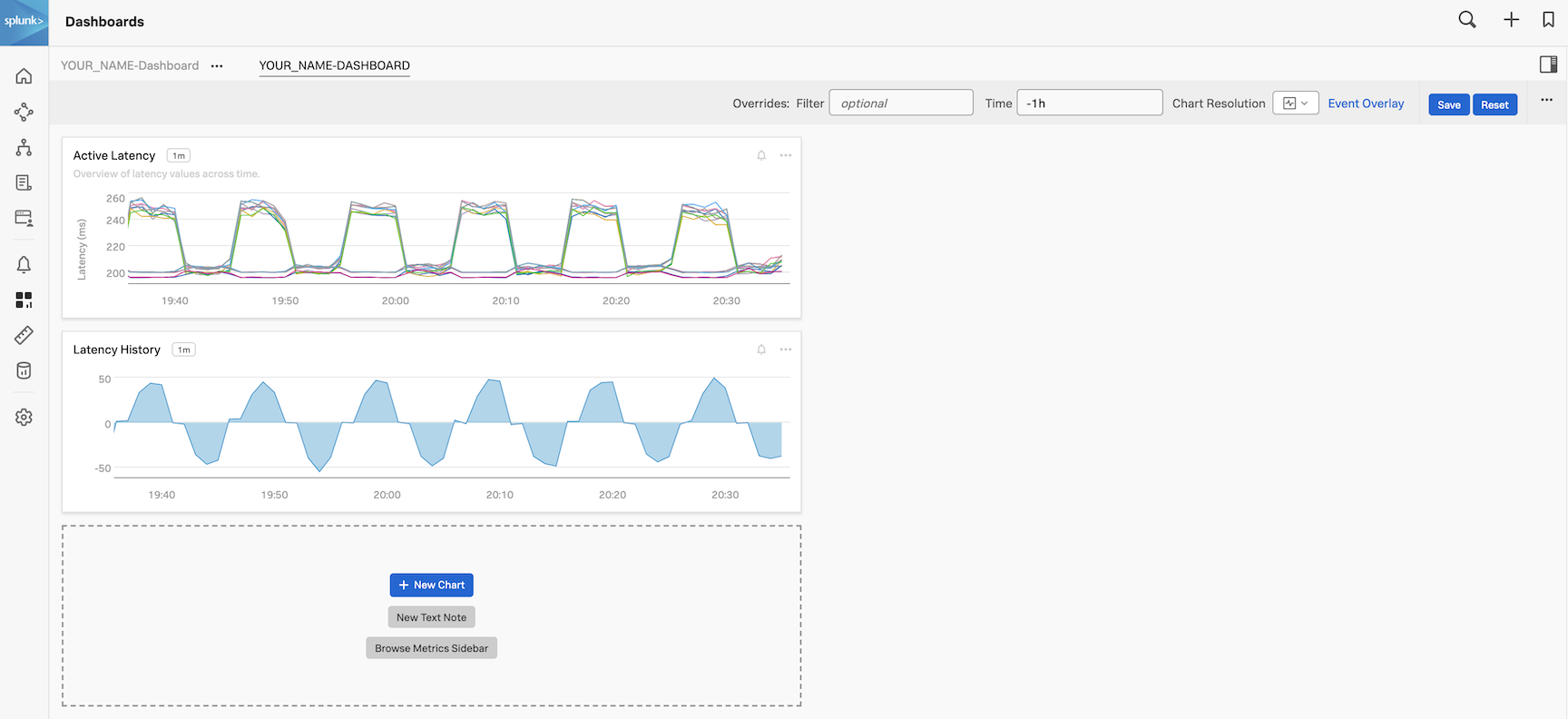 Now let’s quickly add another Chart based on the previous one.
2. Copy and Paste a chart
Click on the three dots ... on the Latency History chart in your dashboard and then on Copy.
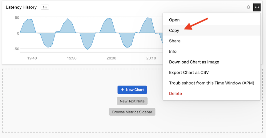
You see the chart being copied, and you should now have a red circle with a white 1 next to the + on the top left of the page.
Click on the plus icon the top of the page, and then in the menu on Paste Charts (There should also be a red dot with a 1 visible at the end of the line).
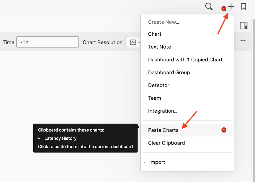
This will place a copy of the previous chart in your dashboard.
3. Edit the pasted chart
Click on the three dots ... on one of the Latency History charts in your dashboard and then on Open (or you can click on the name of the chart which here is Latency History).
This will bring you to the editor environment again.
First set the time for the chart to -1 hour in the Time box at the top right of the chart. Then to make this a different chart, click on the eye icon in front of signal “A” to make it visible again, and then hide signal “C” via the eye icon and change the name for Latency history to Latency vs Load.
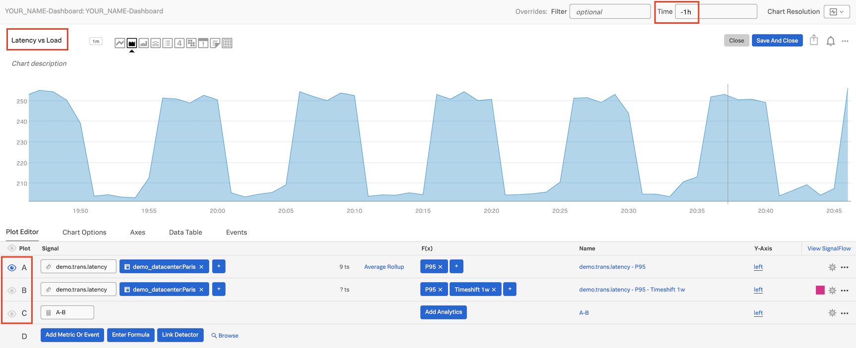
Click on the Add Metric Or Event button. This will bring up the box for a new signal. Type and select demo.trans.count for Signal D.
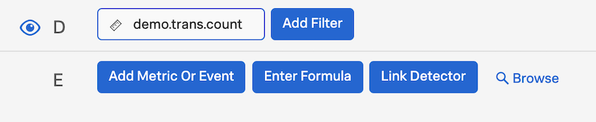
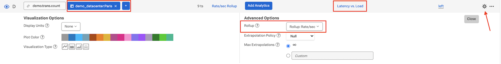
This will add a new Signal D to your chart, It shows the number of active requests. Add the filter for the demo_datacenter:Paris, then change the Rollup type by clicking on the Configure Plot button and changing the roll-up from Auto (Delta) to Rate/sec. Change the name from demo.trans.count to Latency vs Load.
Finally press the Save And Close button. This returns you to your dashboard that now has three different charts!
Let’s add an “instruction” note and arrange the charts!
Adding Notes and Dashboard Layout
1. Adding Notes
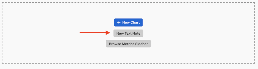
Often on dashboards it makes sense to place a short “instruction” pane that helps users of a dashboard. Lets add one now by clicking on the New Text Note
Button.
This will open the notes editor.
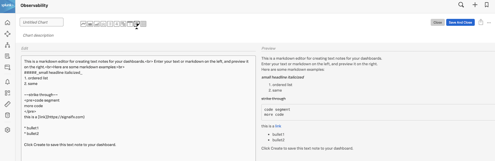
To allow you to add more then just text to you notes, Splunk is allowing you to use Markdown in these notes/panes.
Markdown is a lightweight markup language for creating formatted text using plain-text often used in Webpages.
This includes (but not limited to):
- Headers. (in various sizes)
- Emphasis styles.
- Lists and Tables.
- Links. These can be external webpages (for documentation for example) or directly to other Splunk IM Dashboards
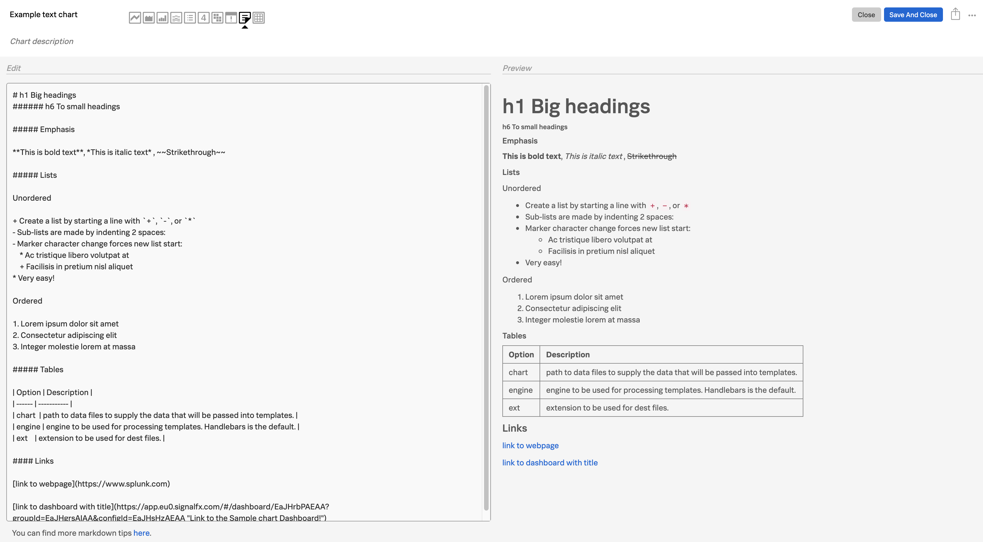
Below is an example of above Markdown options you can use in your note.
# h1 Big headings

###### h6 To small headings

##### Emphasis

**This is bold text**, *This is italic text* , ~~Strikethrough~~

##### Lists

Unordered

+ Create a list by starting a line with `+`, `-`, or `*`
- Sub-lists are made by indenting 2 spaces:
- Marker character change forces new list start:
    * Ac tristique libero volutpat at
    + Facilisis in pretium nisl aliquet
* Very easy!

Ordered

1. Lorem ipsum dolor sit amet
2. Consectetur adipiscing elit
3. Integer molestie lorem at massa

##### Tables

| Option | Description |
| ------ | ----------- |
| chart  | path to data files to supply the data that will be passed into templates. |
| engine | engine to be used for processing templates. Handlebars is the default. |
| ext    | extension to be used for dest files. |

#### Links

[link to webpage](https://www.splunk.com)

[link to dashboard with title](https://app.eu0.signalfx.com/#/dashboard/EaJHrbPAEAA?groupId=EaJHgrsAIAA&configId=EaJHsHzAEAA "Link to the Sample chart Dashboard!")
Copy the above by using the copy button and paste it in the Edit box.
the preview will show you how it will look.
2. Saving our chart
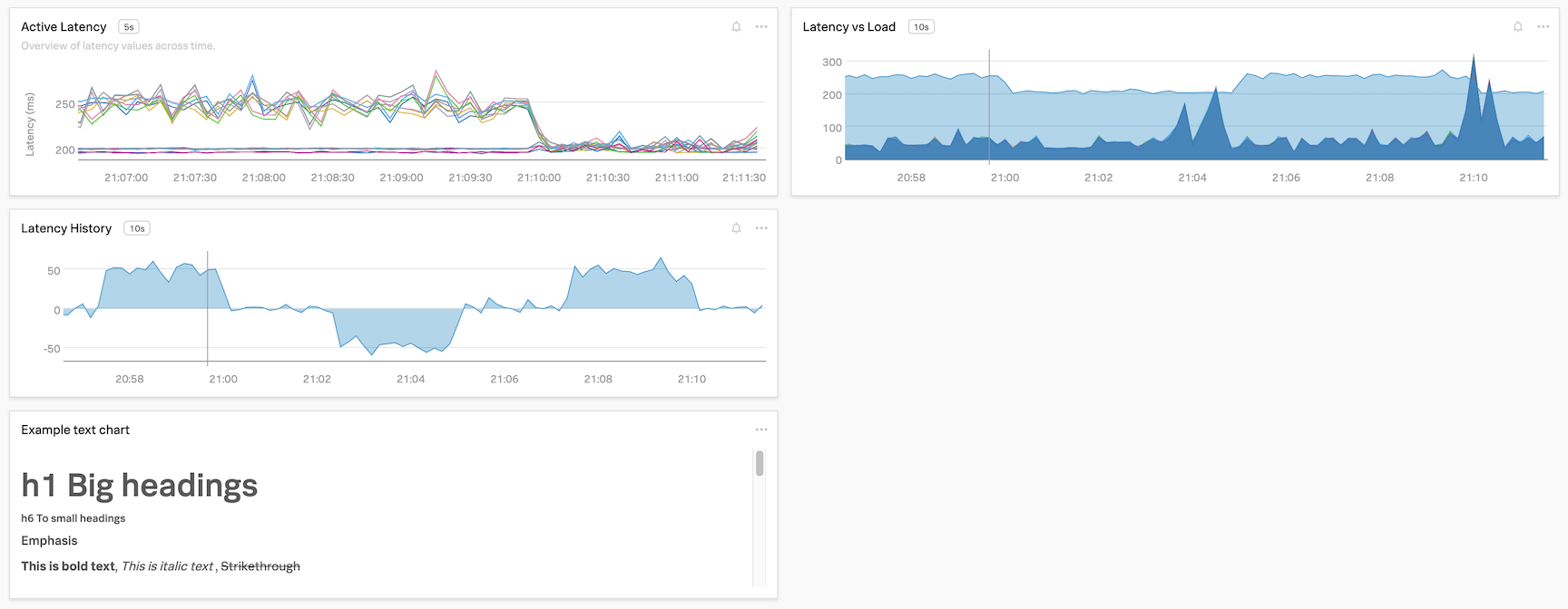
Give the Note chart a name, in our example we used Example text chart, then press the Save And Close Button.
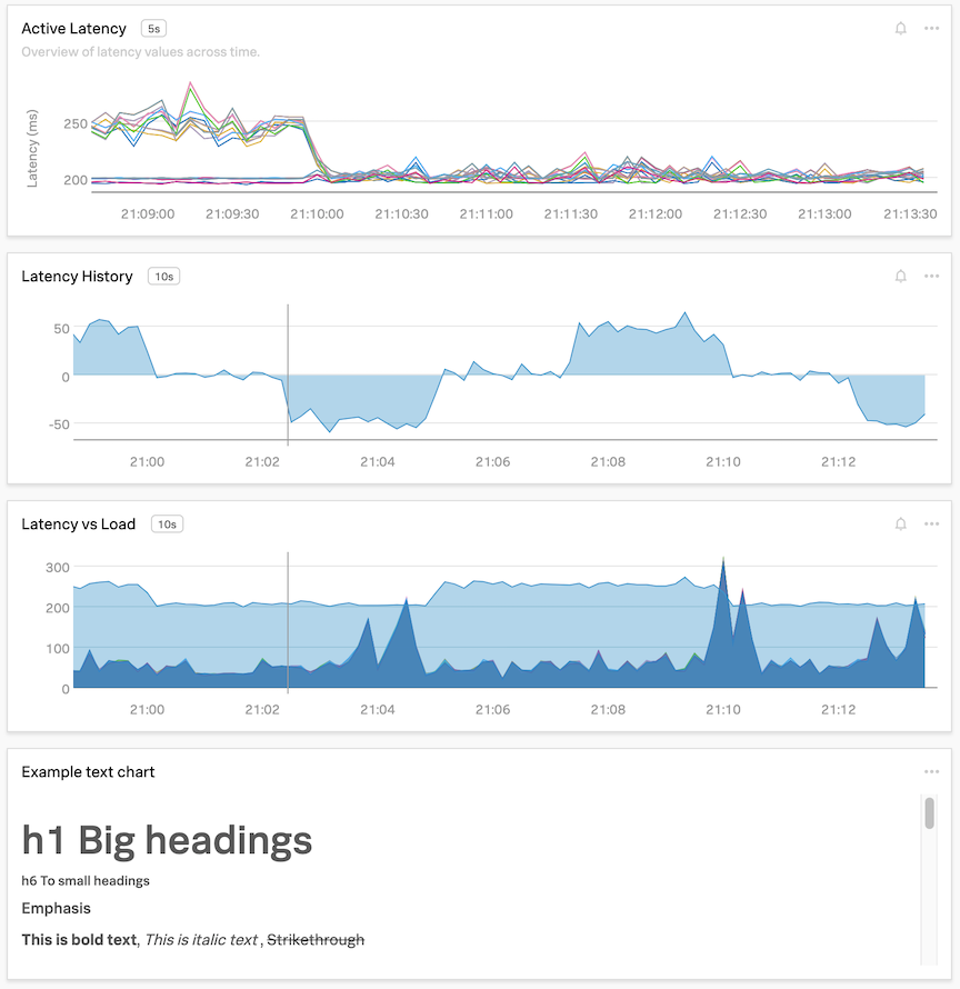
This will bring you back to you Dashboard, that now includes the note.
3. Ordering & sizing of charts
If you do not like the default order and sizes of your charts you can simply use window dragging technique to move and size them to the desired location.
Grab the top border of a chart and you should see the mouse pointer change to a drag icon (see picture below).
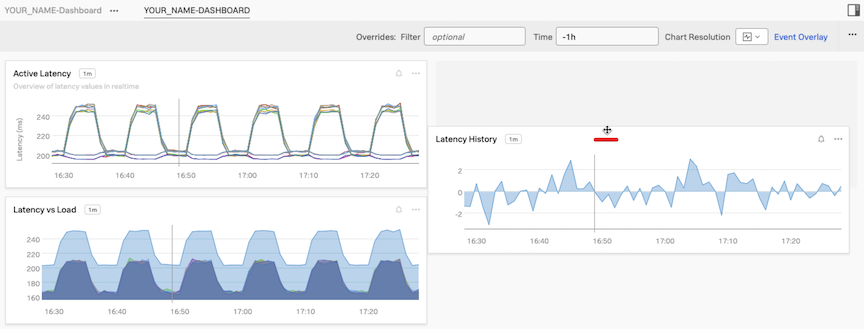
Now drag the Latency vs Load chart to sit between the Latency History Chart and the Example text chart.
You can also resize windows by dragging from the left, right and bottom edges.
As a last exercise reduce the width of the note chart to about a third of the other charts. The chart will automatically snap to one of the sizes it supports. Widen the 3 other charts to about a third of the Dashboard. Drag the notes to the right of the others and resize it to match it to the 3 others. Set the Time to -1h and you should have the following dashboard!
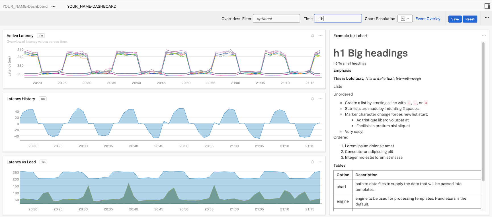
On to Detectors!