Environment Topology

Why This View Matters

The Environment Topology view answers a question every SAP administrator has: “what’s actually talking to what?” Traditional dashboards show events, errors, and aggregates per source — but the shape of how SAP systems integrate with each other (RFC partners, HANA tenant relationships, web traffic boundaries, cross-zone connections) is hidden in those tabular surfaces. This view materializes that shape as an interactive graph drawn from your existing log data — no new ingest, no CMDB integration, no tagging effort required.

Use it to:

• Validate that your topology matches the as-designed architecture (every system shows up; no rogue partners are talking inbound).
• Investigate a single SID’s call surface — who calls it, what does it call, where are the errors concentrated?
• Drill from an edge (a single integration relationship) into the raw events with one click — every edge carries a denormalized SPL filter expression so you can pivot to Splunk’s universal search instantly.
• Onboard a new analyst by giving them a one-page picture of the SAP landscape before they start digging into individual dashboards.
• Spot orphaned IPs / hosts that don’t belong to any known SID — these are typically misconfigured load balancers, scanners, or unauthorized integration partners.

This view replaces the manual hand-drawn architecture diagrams that SAP admin teams typically maintain in slides or wikis. Because it’s data-driven, it stays current as systems are added or retired.

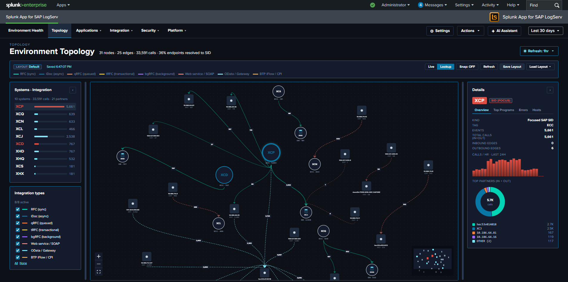
What’s on Screen

The view is laid out in four regions:

Top toolbar — the layout-mode dropdown (Force / Layered / Tree), Refresh button (re-runs the KV Store fetch while preserving saved positions), Save Layout, Load Layout dropdown with the ⚙ Manage Layouts entry, Snap mode toggle, and the saved-layout name chip showing what’s currently loaded.

Left sidebar — two stacked panels. The Systems panel rolls up the inventory (8 systems, total calls, partner count) and lists each focused SID with a per-SID call-volume bar. The Integration types panel is a checkbox list of the eight tracked integration types (RFC sync, iDoc async, qRFC, tRFC, bgRFC, Web service / SOAP, OData / Gateway, BTP iFlow / CPI) — un-ticking a type dims its edges in the canvas without removing them.

Center canvas — the interactive graph itself, rendered with @xyflow/react. Nodes:

• Focused SIDs — large red-ringed circles for the SAP systems your environment is centered around (the high-traffic hubs).
• Secondary SIDs — medium cyan-ringed circles for other internal SAP systems.
• DB-tagged partners — circular discs with a cylinder icon when the partner is a database vendor (HANA, Oracle, MSSQL, Postgres, DB2). HANA systems specifically are tagged when their SID appears as a sap_sid clause on a hana_tenant-type edge — distinct from HANA tenants (which are logical databases inside a HANA system, named after the application SID they back).
• Other partners — rounded squares for non-DB external endpoints (web partners, gateways, generic IPs).

Each SID and DB partner carries a 3-segment health ring painted around its perimeter, showing the proportion of normal (green) / warning (orange) / error (red) calls in the visible time window. Non-DB partners (the rounded squares) carry an equivalent rounded-square perimeter outline. Nodes with no calls or with all calls in a single bucket render as a solid full ring in the dominant color (a healthy node with all-normal calls shows a solid green ring; an idle node still shows green so you can tell the canvas painting succeeded). The classification: edges with errorRate < 10% route their errors to the warning bucket; edges with errorRate ≥ 10% route to the error bucket; everything else is normal. HANA-tagged nodes additionally route WARNING-severity events and slow tenant SQL queries (hana_op_duration_ms > 1000) into the warning bucket as a vendor-specific health signal — these counts are first-class fields on the edge bucket rows, computed at hourly aggregation time from sap:hana:tracelogs.

Right sidebar (selection-driven) — what shows here depends on whether you’ve selected a node or an edge.

When a node is selected, four tabs surface that node’s per-selection context:

• Calls/Hr — bar chart of hourly call volume into the selected node, hardcoded to the last 24 hours regardless of the global time-range picker (this chart’s purpose is “what’s happening RIGHT NOW on this node,” not “what happened over the picker’s window”). For HANA-tagged nodes, an additional roll-up section above the chart shows tenants list, tenant SQL ops, p95/max SQL duration, and auth success/fail counts — derived from incident edges in JS, no extra SPL.
• Programs — top ABAP programs / RFC functions / HANA actions / web URIs invoked on the node, sourced from the gateway, ICM, HANA audit, and webdispatcher logs.
• Errors — categorized error breakdown for the node (HTTP 4xx/5xx, severity ERROR / CRITICAL / FATAL, gateway error_function, ICM transactions). Aggregated by sourcetype + error_kind.
• Hosts — the host(s) backing the SID, with first-seen / last-seen / dc(sourcetype) per host.

When an edge is selected, five tabs surface that edge’s per-call context:

• Overview — endpoint cards (source / direction / target), pre-computed aggregates (call count, error count, error rate, sourcetype), and an inline activity trend chart.
• Activity — full-width stacked-area chart of successful calls + errors over the visible time window.
• Operations — donut chart of the top 10 entities for this edge type (HTTP URIs, RFC programs, HANA actions, HANA trace components).
• Performance — for HTTP edges, latency percentiles (P50 / P95 / Max) and bytes-out plus per-status-class call counts. For RFC, ICM tasks histograms. For HANA, percentile breakdown via transpose 0.
• Errors — top 15 failure modes with error_kind, error_detail, count, and last-seen timestamp.

Selection is mutex — clicking a node clears any selected edge and vice versa, so the right pane never shows mixed context. Clicking empty canvas (the pane) clears both. Each side preserves its own preferred tab independently when you swap between selections.

Bottom panel — Live Activity table showing the top 8 RFC partners by call count for the current time range, each row clickable to drill into the source endpoint’s detail.

MiniMap (bottom-right of the canvas) — drag the cursor inside the minimap to pan the main canvas. Direction follows the cursor: dragging right → main canvas shows more right-side content; dragging down → shows more bottom content. Magnitude is proportional to your cursor delta scaled by the minimap’s viewBox-to-pixel ratio. Single-click does nothing — drag-to-pan is the only minimap interaction.

Where the Data Comes From

The view reads from a time-bucketed KV Store fed by hourly scheduled saved searches. (An earlier design ran six SPL searches on demand every time the view opened, which produced a 5–15 second page load on busy Splunk instances; the data layer was rewritten to the KV Store design described here.)

KV Store collection	Schema	Populated by
logserv_topology_nodes	one row per (canonical entity, hourly bucket); 10 fields including event_count, last_seen	logserv_topology_aggregate_nodes (hourly cron 5 * * * *)
logserv_topology_edges	one row per (edge, hourly bucket); 21 fields including pre-computed response_time_p50/p95/max, icm_tasks_max/avg, hana_op_p95_ms/max, auth_success_count/fail_count, error_count, plus canonical spl_sourcetype + spl_filter_clauses for right-pane drilldowns	logserv_topology_aggregate_edges (hourly cron 5 * * * *)
logserv_topology_inventory	flat (no bucket dimension), keyed by canonical_value; IP / host → SID mapping for retargeting raw IPs to their owning SID node	logserv_topology_aggregate_inventory (hourly cron 5 * * * *)

Two retention searches keep the KV Store sized: logserv_topology_retention (daily 00:30 UTC) trims to 30 days of bucket history; logserv_topology_backfill_* (disabled by default) lets an admin re-populate the 30-day window after a fresh install via Settings → Dashboard Data.

The aggregation searches read from the same six SPL sources as the legacy on-demand path:

Source	What it contributes
sap:abap:gateway	RFC peer/local IPs (P=<peer> / L=<local> fields). The local IP is canonical for IP→SID inventory because it always belongs to this host’s SID.
sap:abap:icm	ICM peer/local IPs for HTTP-side traffic.
sap:hana:tracelogs	HANA host + tenant SID extracted from the source path (/usr/sap/<HANA_SID>/HDB<inst>/<host>/trace/DB_<TENANT_SID>/). Yields the rich HANA-side topology including multi-tenant relationships.
sap:saprouter	Peer hostname extracted from the parens after host <ip>/<service> (<resolved.host>). Provides the inbound edge for external partners.
linux_messages_syslog (osquery cpu_brand subset)	Host inventory: CPU model, RAM, OS, region, AZ, EC2 instance ID. Used to enrich the host-level facts on the Hosts tab.
Default Splunk host field (cross-source fallback)	Picks up hosts that aren’t surfaced in the above.

When you open the view, the React app fetches a time-window slice of these collections via the Splunk Web REST proxy (/en-US/splunkd/__raw/servicesNS/nobody/<APP>/storage/collections/data/<NAME>?query={"bucket_ts":{"$gte":...,"$lte":...}}). The fetch returns in well under a second on production-scale data — orders of magnitude faster than the legacy on-demand path. Per-edge SPL searches still dispatch on demand when you click an edge (the right pane’s 5 tabs each fire one tab-specific query) but they hit pre-narrowed indexes and return quickly.

Self-Derived IP→SID Inventory

The “which IP belongs to which SID” mapping isn’t read from a CMDB or an admin-maintained lookup — it’s self-derived from the same logs you’re already ingesting. The mechanism is a multi-source union SPL with a mvcount(sids)=1 filter: a host whose multiple sourcetypes all agree on a single SAP SID is unambiguously attributed; otherwise it’s marked “unknown.”

Coverage depends on what your data exposes — unique hostname/IP appearances across multiple SAP sourcetypes attribute cleanly, while shared NAT IPs and external partners typically appear as “unknown” nodes (their SAP affiliation isn’t observable from logs alone, or they legitimately don’t belong to any single SID).

In addition to the inventory, the node-aggregation SPL captures every distinct edge endpoint as a node row in its own right — webdispatcher clientip, ABAP gateway peer_ip, and HANA Audit client_ip (excluding loopback). This means external partners that appear only on the receiving side of integration edges still carry real event counts, not zero, even when they don’t have a SID resolution in the inventory.

The inventory itself is extensible per-customer without new ingest: appending another union arm to the inventory aggregation SPL adds a new attribution source. Future arms could include ICM icm_peer_ip, additional CMDB-style lookup tables, or any other field that uniquely associates an IP / host with a SAP SID.

Layout Modes

The LAYOUT dropdown switches between three layout algorithms:

• Force — d3-force directed graph with charge varying by node kind. Best for small-to-medium graphs and exploratory views; the default for first-time viewers.
• Layered — ELK Sugiyama-layered top-to-bottom flow with orthogonal edges and near-zero edge crossings. Best for traffic-flow analysis where you want to see “what flows into what” structurally.
• Tree — ELK mrtree classic top-down tree with hubs at top and spokes radiating downward. Best when the topology is approximately hub-and-spoke shaped.

Both ELK-based modes (Layered + Tree) share the same lazy-loaded ~280 KB elkjs bundle, so adding Tree mode after Layered shipped was a near-zero-cost extension. Force mode remains synchronous (no bundle hit on initial load).

Each layout mode has its own saved-layout slot — saving a layout in Force doesn’t bleed into Layered or Tree. Switching layouts via the LAYOUT dropdown drops the current saved-positions cache so each mode renders fresh from its own algorithm. The Manage Layouts modal (⚙ entry at the top of the Load Layout dropdown) lets you set a per-mode default layout that auto-loads on mount.

Saved Layouts

User-arranged graph layouts are persisted in Splunk KV Store collection logserv_topology_layouts. Each saved layout carries:

• Layout mode — Force / Layered / Tree (so a Force-saved arrangement loads back in Force mode, not Layered)
• Node positions — where you’ve manually placed each node on the canvas
• Panel state — sidebar tab + width
• Viewport — zoom level + pan offset (x, y)
• Enabled integration types — which checkboxes are ticked on the leftbar
• Selected node / edge — what was selected when you saved
• Active right-sidebar tab — Calls/Hr / Programs / Errors / Hosts (node mode) or Overview / Activity / Operations / Performance / Errors (edge mode)
• Snap mode — whether new nodes snap to a grid

Layouts are saved per-user-named — you can save your own variants (“focus on XCQ”, “all DBs”, “external partners only”) and switch between them from the Load Layout dropdown.

The Manage Layouts modal (⚙ entry at the top of the Load Layout dropdown) is where two cross-browser preferences live:

• Per-mode default layout — pick one saved layout per mode (Force / Layered / Tree) to auto-load on mount when you’re using that mode. Each mode section in the modal has its own radio list of mode-matching layouts plus a “(no default)” option.
• Default layout mode — tick the Open in this mode by default checkbox on one of the three sections to declare which mode the dashboard should open in on next login. The checkbox is mutex across the three sections (or none — “no explicit default” leaves the dashboard opening in Force mode). Ticking the checkbox also switches the active mode immediately so you can see what the default-on-next-login experience will look like.

Both preferences are persisted to Splunk KV Store keyed by Splunk username (collections logserv_topology_layout_defaults and logserv_topology_active_mode). Browser localStorage is used as a fast-mount cache mirror, so on a fresh browser the choices hydrate from KV Store on first paint. If you pick defaults in Chrome and open the topology in Firefox, you’ll see the same defaults the next time you log in to the same Splunk instance. When no defaults are stored, the dashboard opens in Force mode with no auto-loaded layout.

Data Refresh Cadence

The topology data layer is populated by three hourly scheduled saved searches that write to the KV Store:

• logserv_topology_aggregate_nodes — cron 5 * * * *, rolls up event activity per (canonical entity, hour bucket)
• logserv_topology_aggregate_edges — cron 5 * * * *, rolls up call counts + per-type aggregates (HTTP latency p50/p95/max, RFC saturation, HANA SQL latency, etc.)
• logserv_topology_aggregate_inventory — cron 5 * * * *, rebuilds the unambiguous IP/host → SID mapping

So the KV Store gets a new bucket every hour at H+5. The view re-reads the KV Store:

• On initial page load
• On global TimeRange picker change
• When the user clicks the toolbar’s Refresh button (useful right after dispatching a backfill saved search)
• When the user selects a different node (re-runs the per-node detail-panel SPL via on-demand useSearch — independent of the KV Store layer)

There is no client-side auto-polling. The previous Live | Lookup mode toggle was removed in session 044 — the 30-second polling cadence was a leftover from the pre-session-035 on-demand SPL data layer, and after the move to hourly KV Store aggregation, ~119 of every 120 ticks returned byte-identical data. The hourly cron is what governs data freshness now; tightening the cron schedule (e.g., to */15 * * * *) is the right lever if a customer needs sub-hour data freshness, at the cost of more search-job dispatches.

What to Look For

• Health rings with prominent orange or red segments — a SID showing >25% red (error bucket) is a system whose external integrations are systematically failing. Click into the node and the Errors tab to see which specific edges are degraded.
• Unknown nodes with high edge weight — an “unknown” SID with hundreds of calls/hr is either a misconfigured CMDB entry on our side, OR an unauthorized partner that nobody documented. Both warrant investigation.
• Asymmetric edge counts — an edge showing many calls one direction but very few the other usually means one side is the caller (RFC client) and the other is the callee (RFC server). Use the Operations tab to confirm which.
• Orphan SIDs — a node with no edges is a system that’s running but not integrated with anything else. May be a quiet test system, or a system whose integration partners aren’t monitored.
• HANA tenants drifting from their HANA system — multi-tenant HANA produces edges from the parent system to each tenant. Missing tenant edges indicate either tenant outage or audit-log gap. The HANA-tagged DB partners specifically use slow tenant SQL queries (>1000 ms) as a warning signal; a tenant lighting up with orange in its ring after a deploy points at slow-query regressions.
• Unexpected external partners — saprouter peer_hostname entries that don’t match the documented partner list are the strongest signal of an unauthorized external integration.
• Edge errors clustered on one sourcetype — clicking an edge and reading the Errors tab can reveal that 90% of failures are 4xx (client-side, not your problem) vs 5xx (server-side, your problem). The edge bucket schema pre-computes per-status-class counts so the Performance tab loads instantly.
• Host counts on the Hosts tab — a SID showing 3 hosts when you expected 2 may indicate a stale forwarder / VM that should have been decommissioned.

Notes

• The view’s URL slug is /integration-topology (historical — the user-visible label was changed from “Integration Topology” to “Environment Topology”, but the URL slug + code identifiers stayed stable so existing bookmarks + saved-layout records remain valid).
• Layout persistence works across browser tabs and across Splunk Web sessions — your KV Store records survive Splunkd restarts.
• Layouts are saved per Splunk user — every KV Store record is keyed by <username>::<slug>, so different users have completely separate records and can’t overwrite each other’s layouts. If the same user edits the topology in two browser tabs concurrently, the tabs race each other and last-tab-save wins (multi-tab edit-collision protection is planned for a future release).
• The minimap supports drag-only panning. Single-click and scroll-zoom inside the minimap rectangle are intentionally inert — drag is the one interaction.